


How much does televised campaign advertising affect election outcomes in the United States? This has been a pertinent question since the first televised advertisements were aired during a 1950 Connecticut Senate election and then by President Dwight Eisenhower’s 1952 campaign (Benoit Reference Benoit2018). Answering this question helps illuminate the motivations behind voting behavior, the influence of mass communication on the electorate, and how much candidates’ resources and messages can help them win elections. Moreover, the aggregate effect of televised advertising may determine the actual winner in at least some races, thereby affecting the composition of government and the direction of public policy.
Political campaigns spend a great deal of money on television advertising. According to Fowler, Ridout, and Franz (Reference Fowler, Ridout and Franz2016), over $2.75 billion was spent to air over 4.25 million ads in the 2015–2016 election cycle. This includes about 1 million airings in the presidential race, 1 million airings in Senate races, 620,000 airings in House races, and 1.25 million airings in other races at the state and local levels. Spending on television advertising constitutes about 45% of a typical congressional campaign’s budget (Jacobson and Carson Reference Jacobson and Carson2019).
Research on televised political advertising has made significant progress in estimating its influence on voting behavior (for overviews, see Fowler, Franz, and Rideout Reference Fowler, Franz and Rideout2016; Goldstein and Ridout Reference Goldstein and Ridout2004; Jacobson Reference Jacobson2015). Studies have found associations between television advertising and individual vote intentions, aggregate vote shares, or both (e.g., Huber and Arceneaux Reference Huber and Arceneaux2007; Rideout and Franz Reference Ridout and Franz2011; Sides and Vavreck Reference Sides and Vavreck2013; Spenkuch and Toniatti Reference Spenkuch and Toniatti2018). In presidential general elections, the persuasive influence of television advertising appears to be larger than that of other electioneering such as canvassing or mail, the influence of which is quite small, even zero (Kalla and Broockman Reference Kalla and Broockman2018).
But there are significant limitations to what we know about the effects of televised campaign advertising on election outcomes. Most importantly, the extant literature is almost entirely focused on presidential general elections (e.g., Gordon and Hartmann Reference Gordon and Hartmann2013; Johnston, Hagen, and Jamieson Reference Johnston, Hagen and Jamieson2004; Shaw Reference Shaw2006; Sides and Vavreck Reference Sides and Vavreck2013; Sides, Tesler, and Vavreck Reference Sides, Tesler and Vavreck2018; Spenkuch and Toniatti Reference Spenkuch and Toniatti2018). Only a few studies have examined advertising effects in Senate elections (Fowler, Ridout, and Franz Reference Fowler, Ridout and Franz2016; Goldstein and Freedman Reference Goldstein and Freedman2000; Jacobson Reference Jacobson1975; Ridout and Franz Reference Ridout and Franz2011; Wang, Lewis, and Schweidel Reference Wang, Lewis and Schweidel2018) or House elections (Hill et al. Reference Hill, Lo, Vavreck and Zaller2013; Jacobson Reference Jacobson1975).Footnote 1 Just two studies have examined gubernatorial elections and both focus on survey-based vote intentions rather than election results (Gerber et al. Reference Gerber, Gimpel, Green and Shaw2011; Hill et al. Reference Hill, Lo, Vavreck and Zaller2013). To our knowledge, there has been no published research on the effect of advertising in down-ballot state-level races, such as elections for state Attorney General. And, most importantly, no study has used a comparable, credible research design to study advertising effects across multiple levels of office. The most relevant prior studies compare presidential and Senate elections (Fowler, Ridout, and Franz Reference Fowler, Ridout and Franz2016; Jacobson Reference Jacobson1975; Ridout and Franz Reference Ridout and Franz2011) and find that advertising in Senate elections appears to have larger effects on election outcomes than does advertising in presidential elections. This paucity of studies illustrates the conclusion of Kalla and Broockman (Reference Kalla and Broockman2018), who, after canvassing the available experiments on persuasion in general election campaigns, argue that “more evidence” on televised advertising “would clearly be welcome” (163). We seek to provide that evidence.
Campaign advertisements provide information to voters that may change the balance of considerations they hold about candidates in a given contest. As the balance shifts, citizens may change their views of the candidates (persuasion) or change their mind about whether to vote at all (mobilization). If advertising affects election outcomes mainly through persuasion at the individual level, it should have larger effects in down-ballot races than in presidential races. This is because voters know less and have weaker opinions about down-ballot candidates relative to presidential candidates. But if advertising works mainly through mobilization, potentially altering the partisan composition of the electorate, voters’ decisions to stay home or turn out should affect all races on the ballot similarly. If so, there should be little heterogeneity across offices in the effect of ads on election outcomes.
We test these expectations by examining the effects of broadcast television advertising on election outcomes in the five presidential elections from 2000 to 2018 and also in 331 US Senate elections, 226 gubernatorial elections, 3,859 US House elections, and 237 other state-level elections during this period. In total, we examine over 4,500 different races. To address the possibility that campaigns may place ads in media markets where they expect to do well (Erikson and Tedin Reference Erikson and Tedin2019, 250), we employ research designs that strengthen the causal interpretation of our findings, including time-series cross-sectional models with a difference-in-differences design (Angrist and Pischke Reference Angrist and Pischke2009) and a border-discontinuity design (Spenkuch and Toniatti Reference Spenkuch and Toniatti2018).
We find that the effect of ad airings is much larger in down-ballot elections than in presidential elections. The apparent effect of an individual airing is two to four times larger in gubernatorial, US House, and US Senate elections and 10 to 19 times larger in other statewide races, compared with presidential elections.
We also provide evidence that persuasion is the primary mechanism through which these differing effects of advertising emerge. Drawing on surveys of hundreds of thousands of voters across eight election cycles, we show that voters have less information and weaker opinions about the candidates in down-ballot races than about presidential candidates and that in these down-ballot races television advertising is more strongly associated with voters’ knowledge of the candidates, evaluations of the candidates, and ideological congruence with the candidates than it is in presidential races. By contrast, we find less evidence for another possible mechanism: that television advertising affects election outcomes by changing the partisan composition of the electorate. Drawing on administrative data from six different election cycles, we show that advertising is not consistently associated with the relative turnout of Democrats and Republicans. Moreover, we find that ads for one race do not substantially “spill over” and affect outcomes at another level of office, as would be true if advertising altered the partisan composition of the voters in any election year.
Our paper has several implications for the study of voting behavior and elections. Despite increasing partisan loyalty among American voters, some voters still respond to television advertising. This is particularly true in down-ballot elections. Indeed, while television advertising is likely to swing only very close presidential elections, infusions of television advertising could swing a larger number of close down-ballot elections. Thus, the effort that candidates, political parties, and outside groups invest in raising money for, producing, and airing television advertising pays dividends. Mass communication in electoral campaigns matters, even in a more polarized electorate.
Theoretical Motivation
Does television advertising in US elections affect election outcomes? And should its effect vary across levels of office? Drawing on literatures in psychology, political science, economics, and political communication, we assemble a set of expectations for both questions.
Campaign advertising can persuade voters if it provides novel information that affects their attitudes about one or both candidates. Prior research on attitude change shows that people can be susceptible to persuasion, but that there are many obstacles to changing someone’s mind (e.g., DellaVigna and Gentzkow Reference DellaVigna and Gentzkow2010; Petty, Priester, and Wegener Reference Petty, Priester, Wegener, Wyer and Srull2014; Sears and Kosterman Reference Sears, Kosterman, Shavitt and Brock1994). This well-established idea is central to theories of information processing in political science. For one, Zaller (Reference Zaller1992) argues that attitude change in response to information is conditional on partisanship and other predispositions (“partisan resistance”) as well as the number of existing considerations that someone has about an attitude object (“inertial resistance”). For another, Lodge and Taber (Reference Lodge and Taber2013) argue that once people think about a political object, that object has an “affective tag” (a positive or negative feeling) stored in memory, which then influences subsequent information-processing and leads to “motivated reasoning.” Both accounts suggest that persuasion is possible, but when people have relevant prior attitudes, and especially strongly held attitudes, they are less likely to change their attitudes in response to new information.
This pattern suggests more potential for persuasion in down-ballot races, where people have thought less about the candidates and have fewer stored considerations and weaker affective tags, if any. As Delli Carpini and Keeter (Reference Carpini, Michael and Keeter1996) show, Americans are more familiar with national political figures, such as the president and vice-president, than with figures like US Senators. Indeed, the percentage of Americans who could name both Senators declined between 1947 and 1989, even as the percentage who could name the vice-president increased. Likewise, Hopkins (Reference Hopkins2018) shows that the percentage of Americans who can name their governor declined from 87% in 1947 to 66% in 2007. Hopkins also finds that Americans could supply less information about governors than presidents when asked to describe them, and they were less likely to search the Internet for information about governors than presidents. These declines are likely linked to the decreasing amount of news coverage of state and local politics (Hayes and Lawless Reference Hayes and LawlessForthcoming). Research on congressional elections also finds differences in knowledge across levels of office. In particular, a larger percentage of Americans can recall and recognize the names of US Senate candidates than US House candidates (Jacobson and Carson Reference Jacobson and Carson2019). Here again, knowledge of congressional candidates is linked to how much local news covers congressional campaigns (Hayes and Lawless Reference Hayes and Lawless2018).
These informational and attitudinal asymmetries across levels of political office imply that new information—such as in television advertising—should more strongly influence views of down-ballot candidates than views of presidential candidates.Footnote 2 The persuasive potential of campaigns and campaign advertising is evident in previous research. Campaigns provide information to voters, who become better able to name candidates (Elms and Sniderman Reference Elms, Sniderman, Brady and Johnston2006; Jacobson Reference Jacobson, Brady and Johnston2006) and identify where the candidates stand on political issues (Alvarez Reference Alvarez1998; Franklin Reference Franklin1991; Johnston, Hagen, and Jamieson Reference Johnston, Hagen and Jamieson2004; Patterson and McClure Reference Patterson and McClure1972). Television advertising specifically contributes both to informational gains (Freedman, Franz, and Goldstein Reference Freedman, Franz and Goldstein2004) and changes in attitudes toward the candidates (Coppock, Hill, and Vavreck Reference Coppock, Hill and Vavreck2020; Freedman and Goldstein Reference Freedman and Goldstein1999; Huber and Arceneaux Reference Huber and Arceneaux2007; Johnston, Hagen, and Jamieson Reference Johnston, Hagen and Jamieson2004; Ridout and Franz Reference Ridout and Franz2011).Footnote 3 Moreover, Huber and Arceneaux (Reference Huber and Arceneaux2007) show that changes in attitudes toward the candidates—that is, persuasion—are an important mechanism by which television advertisements influence vote intentions. This potential for persuasion is in line with the strategies of candidates themselves, who air advertising primarily on programs with audiences containing many swing voters (Lovett and Peress Reference Lovett and Peress2010).
Synthesizing this prior work on information, persuasion, and advertising leads to several expectations. We expect that television advertising has a larger effect on election outcomes in down-ballot races for Congress, governor, and other statewide offices than in presidential races. In terms of pathways for this effect, we expect that voters are less likely to have opinions about down-ballot candidates and, when they do have opinions, these opinions are weaker than their opinions about presidential candidates. Therefore, we expect that television advertising has a larger effect on voters’ knowledge and attitudes about down-ballot candidates compared with presidential candidates. Evidence for these latter two expectations will suggest that persuasion is a primary mechanism by which advertising affects election outcomes.
A contrasting expectation is that television advertising affects outcomes mainly through its effect on whether partisans turn out to vote. Although political advertising does not appear to have a significant effect on overall turnout (Ashworth and Clinton Reference Ashworth and Clinton2007; Krasno and Green Reference Krasno and Green2008; Lovett and Peress Reference Lovett and Peress2010; Spenkuch and Toniatti Reference Spenkuch and Toniatti2018; but see Green and Vavreck Reference Green and Vavreck2008), it could affect the partisan composition of the electorate if candidates’ ads mobilize their own partisans and demobilize their opponent’s partisans in roughly equal amounts. Prior research has found that the partisan composition of the electorate is associated with partisan campaign activity aggregated across levels of office (McGhee and Sides Reference McGhee and Sides2005) as well as national party spending (Holbrook and McClurg Reference Holbrook and McClurg2011). Most relevant to this study is Spenkuch and Toniatti (Reference Spenkuch and Toniatti2018), who find that presidential television advertising is associated with the partisan composition of the electorate in the 2004–12 elections.
If advertising matters mainly through partisan mobilization, then, contrary to the first expectation, advertising should have a similar relationship to election outcomes across levels of office. Assuming that partisans vote for their party’s candidate at similar rates across levels of office, any shifts in partisan turnout induced by advertising should affect candidates up and down the ballot in roughly equal amounts. We test for partisan mobilization in two ways: by examining the relationship between advertising and partisan turnout across several election cycles and by examining the relationship between advertising at one level of office and outcomes at other levels. Any “spillover” across levels of office suggests that ads affect partisan turnout and thus affect races other than the one the ads are targeting.
Data and Research Design
To evaluate the effect of political advertising, we built a panel dataset of election returns and advertising data at the county level that substantially extends similar datasets in other work (e.g., Fowler, Ridout, and Franz Reference Fowler, Ridout and Franz2016; Ridout and Franz Reference Ridout and Franz2011; Shaw Reference Shaw2006; Sides, Tesler, and Vavreck Reference Sides, Tesler and Vavreck2018; Sides and Vavreck Reference Sides and Vavreck2013). This dataset’s considerable temporal and geographic scope, alongside a credible research design, provides a rigorous test of the causal effect of advertising on thousands of election outcomes.
We assembled 2000–2018 national, state, and local election returns from various sources. For presidential, senate, and gubernatorial elections, we used data from CQ’s Voting and Elections Collection. For House elections during this period, we used data from the Atlas of U.S. Elections (Leip Reference Leip2016), which break the congressional election returns down by county.Footnote 4 For other state offices (i.e., attorney general and treasurer), we used crowd-sourced county-level data from OurCampaigns.com.Footnote 5
Our primary treatment variable is the net Democratic advantage in the number of broadcast television ad airings in a county over the last two months (64 days) of the campaign. Similar measures have been used in prior research on advertising effects (e.g., Franz and Ridout Reference Franz and Ridout2007; Lovett and Peress Reference Lovett and Peress2010; Spenkuch and Toniatti Reference Spenkuch and Toniatti2018). To be sure, this measure does not capture all advertising, an increasing percentage of which is aired on local cable outlets or online. But broadcast television advertisements constituted the vast majority of campaign advertising during this period (Fowler, Ridout, and Franz Reference Fowler, Ridout and Franz2016).
We calculate the net Democratic advertising advantage by taking the difference between the number of Democratic and Republican ad airings for a particular race in each media market using advertising data obtained under license from the Wesleyan Media Project and the Wisconsin Advertising Project (Fowler, Franz, and Ridout Reference Fowler, Franz and Ridout2020).Footnote 6 These data include the top 75 media markets in the 2000 election cycle, the top 100 markets in the 2002, 2004, and 2006 cycles, and all 210 media markets since 2008.Footnote 7 Figure 1 displays the net Democratic ad advantage in each media market for an illustrative set of offices and years. It shows not only the comprehensiveness of our data but how much advertising volume varies across offices and geography.

Figure 1. Democratic Advertising Advantage (in 100s of ads) across Geography in an Illustrative Set of Offices and Years
Note: Positive (bluer) values show a pro-Democratic advantage and negative (redder) values show a pro-Republican advantage.
We include all general election advertising supporting the Democratic and Republican candidates in each race, including ads aired by the candidate’s campaign, parties, and outside groups.Footnote 8 Our focus on advertising in the last two months of the campaign reflects the extant finding that ads aired closer to Election Day are more effective than ads aired earlier in the election cycle (e.g., Sides, Tesler, and Vavreck Reference Sides, Tesler and Vavreck2018; Sides and Vavreck Reference Sides and Vavreck2013).Footnote 9
One limitation of this measure is that it does not account for the size of the television audience that could have seen each ad airing. However, counts of ad airings are highly correlated with measures, such as gross ratings points, that do attempt to account for the number of people possibly exposed.Footnote 10
We use two parallel research designs to estimate the causal effect of television advertising on election outcomes. The first design includes all US counties in the media markets contained in the advertising data (e.g., all counties starting in 2008 and a subset of counties before that). We include either county fixed effects to account for time-invariant confounders in each county or a lagged outcome variable in lieu of county fixed effects.Footnote 11 These account for the overall partisan orientation of each county. We also include state-year fixed effects to control for time-varying confounders at the state and national levels (Fowler and Hall Reference Fowler and Hall2018; de Benedictis-Kessner and Warshaw Reference de Benedictis-Kessner and Warshaw2020). The state-year fixed effects account for trends in the political preferences of each state across election years, such as the pro-Republican trend in Ohio or the pro-Democratic trend in Arizona. They also account for race-specific dynamics in each state, such as the strength of the candidates and any incumbency advantage. In our analysis of congressional districts, we use district-year fixed effects to account for the strength of the candidates in each race. Thus, this research design isolates the effects of advertising from other aspects of candidates’ quality and spending.Footnote 12
Although this panel design addresses a host of possible confounders, it may miss the effect of unobserved time-varying confounders at the media market or county levels that could bias our estimates. In particular, campaigns could be strategically targeting their spending in areas of a state where they expect to do well by using information, such as internal polls, that is unavailable to researchers.
Our second research design accounts for this possibility by restricting the sample to counties in the same state that are adjacent to one another but on different sides of the border of a media market. Spenkuch and Toniatti (Reference Spenkuch and Toniatti2018) use this design to study the effects of television advertising in the 2004–2012 presidential elections. Similarly, Huber and Arceneaux (Reference Huber and Arceneaux2007) use media market boundaries to study the effects of television advertising in the 2000 presidential election. Other studies have used discontinuities in treatment exposure across county or state boundaries to study the incumbency advantage (Ansolabehere, Snowberg, and Snyder Reference Ansolabehere, Snowberg and Snyder2006) and the effects of policies like Medicaid expansion and right-to-work laws (e.g., Clinton and Sances Reference Clinton and Sances2018; Feigenbaum, Hertel-Fernandez, and Williamson Reference Feigenbaum, Hertel-Fernandez and Williamson2018).
The intuition behind the border county design is that within a state, adjacent counties that straddle the border of a media market are likely to be similar to one another except that they are on different sides of the media market boundary and therefore may be exposed to different levels of television advertising. Moreover, this variation in advertising spending is plausibly exogenous to characteristics of these border counties. It seems unlikely that advertising is targeted based on the characteristics of specific border counties, especially because the counties on media market boundaries exclude the urban cores of most media markets. For evidence that border county designs achieve balance on many characteristics of counties that could also affect election outcomes, see Spenkuch and Toniatti (Reference Spenkuch and Toniatti2018).
To illustrate this design, Figure 2 shows the border counties in Pennsylvania (shaded in gray). It confirms that most major cities (e.g., Philadelphia, Pittsburgh, Erie, and Scranton) are not in border counties. The adjacent counties that do lie along media market borders tend to be similar to one another. For example, Indiana and Cambria counties are adjacent to each other along the boundary between the Pittsburgh and Johnstown-Altoona media markets. Both counties are largely rural areas where Mitt Romney received about 58% of the vote in the 2012 presidential election.

Figure 2. Illustration of the Border Counties Design in Pennsylvania
Note: The dark lines indicate media market boundaries. The shaded counties, which lie along a media market boundary next to another county in Pennsylvania, are the ones included in the border county sample.
To execute the border county design, we match each county in a state with every other adjacent county that lies on the other side of a media market boundary. The unit of analysis becomes the border county pair, with the two counties on opposite sides of a media market boundary. Thus, a particular county could be in this sample multiple times if it borders multiple counties in this fashion. For this reason, the overall sample size is larger in this design than in the first design.Footnote 13 In analyzing this sample of border counties, we include county fixed effects to account for time-invariant confounders in each county. Crucially, we also include year-specific fixed effects for each pair of border counties. This accounts for the effect of any year-specific unobserved confounders in each border-pair of counties, such as trends in their partisanship or ideology. Thus, only confounders that vary between border counties within a particular election cycle could bias our results using this design. While it is impossible to rule out these confounders, there appears to be no correlation between changes in political advertising and border counties’ time-varying observable characteristics (Spenkuch and Toniatti Reference Spenkuch and Toniatti2018).
To test the assumption that there are no time-varying confounders, typically called the parallel trends assumption, we examined whether future values of television advertising appear to have a significant effect on current outcomes. For both designs, we find that future advertising has no effect on election results (see Appendix B). The fact that both research designs generally pass this “placebo test” suggests that time-varying confounders are not biasing our results. Overall, we believe that the “border county design” is more rigorous than the “all counties” design. But it relies on a much smaller set of counties and could have less external validity. As a result, we use both designs throughout the analysis.
Table 1 shows summary statistics of advertising across offices in all counties and in border county pairs (in hundreds of ads) across 2000–2018. Our treatment variable—the Democratic advertising advantage in the last two months before the election—captures the balance of ads favoring each of the opposing major-party candidates. On average, there is considerable balance such that the mean Democratic advantage is close to 0 in most levels of office other than presidential elections. In presidential elections, Democrats have a modest advantage on average, driven in particular by their advantages in the 2004, 2008, and 2016 elections. But there is considerable variation both across counties and within counties and border county pairs.Footnote 14 This variation is particularly large in races for president, Senate, and Governor, where there is more advertising overall.
Table 1. Summary Data on Broadcast Television Advertising 2000–2018
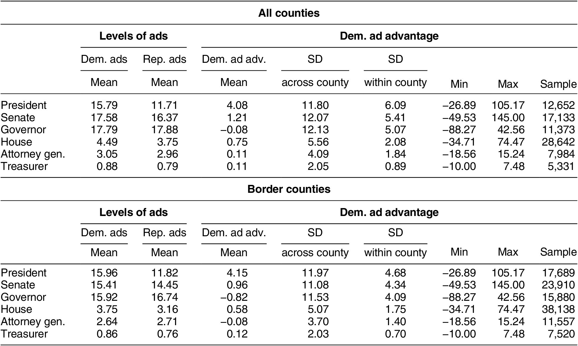
Note: This table shows the average numbers of Democratic and Republicans ads (in 100s) at the county-level over the last two months of the campaign and various statistics on the Democratic advertising advantage at the county-level over the last two months of the campaign. The sample in the top panel includes all counties with elections for each office, and the sample in the bottom panel includes all border county pairs with elections for each office.
Advertising Effects in Presidential Elections
We begin by examining the effects of advertising on the Democratic candidate’s major-party vote share in presidential elections between 2000 and 2016. The first four columns of Table 2 show the results of regression models using all counties where we have advertising data. The first column shows a naive model with just fixed effects for year. This model suggests that a 100-airing advantage yields an additional 0.158 percentage points of vote share. The next column shows the results of a model with year and county fixed effects. The county fixed effects, which address time-invariant confounders, dramatically decrease the estimated effect to 0.043 points, or about four hundredths of a percentage point. The third column shows the results of a model that includes state-year fixed effects and a lagged outcome variable. In this model, a 100-airing advantage for the Democratic candidate is associated with a 0.037-point increase in vote share over the candidate’s vote share in the previous election. The fourth column includes state-year fixed effects, which address time-varying confounders at the state-level as well as county fixed effects. Here, the same advantage is associated with a 0.027-point increase in vote share.
Table 2. The Effects of Television Advertising in Last Two Months of Presidential Elections (2000–2016)

Note: The treatment variable is Democratic ad advantage in terms of hundreds of ads. Standard errors are clustered by county and DMA-year in the left panel and by county and DMA border-year in the right panel. *p < 0.05; **p < 0.01.
The next three columns show the estimated effects of presidential ad airings among pairs of counties along media market borders. In the model that includes state-year fixed effects and a lagged outcome variable, a 100-airing advantage for the Democratic candidate is associated with a 0.027-point increase in vote share (column 5). Including state-year fixed effects and county fixed effects produces an estimate of 0.020 points (column 6). Including border-pair-year fixed effects and county fixed effects produces an estimate of 0.018 points (column 7).Footnote 15
These results show that a more stringent modeling strategy produces a smaller effect of televised advertising on presidential election outcomes. This illustrates the importance of either employing fixed effects or isolating border counties (or both) to avoid overstating the effect. It also bolsters a causal interpretation of our results that we recover similar estimates with two different identification strategies. Ultimately, televised advertising in presidential elections appears to have a modest but detectable relationship to vote share, as previous literature has found.Footnote 16
Our results also place a rough upper bound on the real-world effects of advertising in presidential general elections. Assuming that the effects of ads are linear, our findings imply that moving from three standard deviations below the average advertising advantage to three standard deviations above the average (a 6-standard-deviation shift) within border pairs would lead to a 0.5-point change in two-party vote share.
Advertising Effects in Down-Ballot Elections
How does the effect of televised advertising in presidential elections compare with its effects in other types of elections? The top panel of Table 3 shows the effect of advertising across different offices using the all county sample. Here, we use the specification with both county and state-year fixed effects (column 4 of Table 2). The bottom panel of Table 3 shows the effect of advertising across different offices using the border county sample and the specification with county and adjacent-county-year fixed effects (column 7 of Table 2).Footnote 17
Table 3. Effects of Aggregate Television Advertising in Last Two Months of Election across Offices (2000–2018)
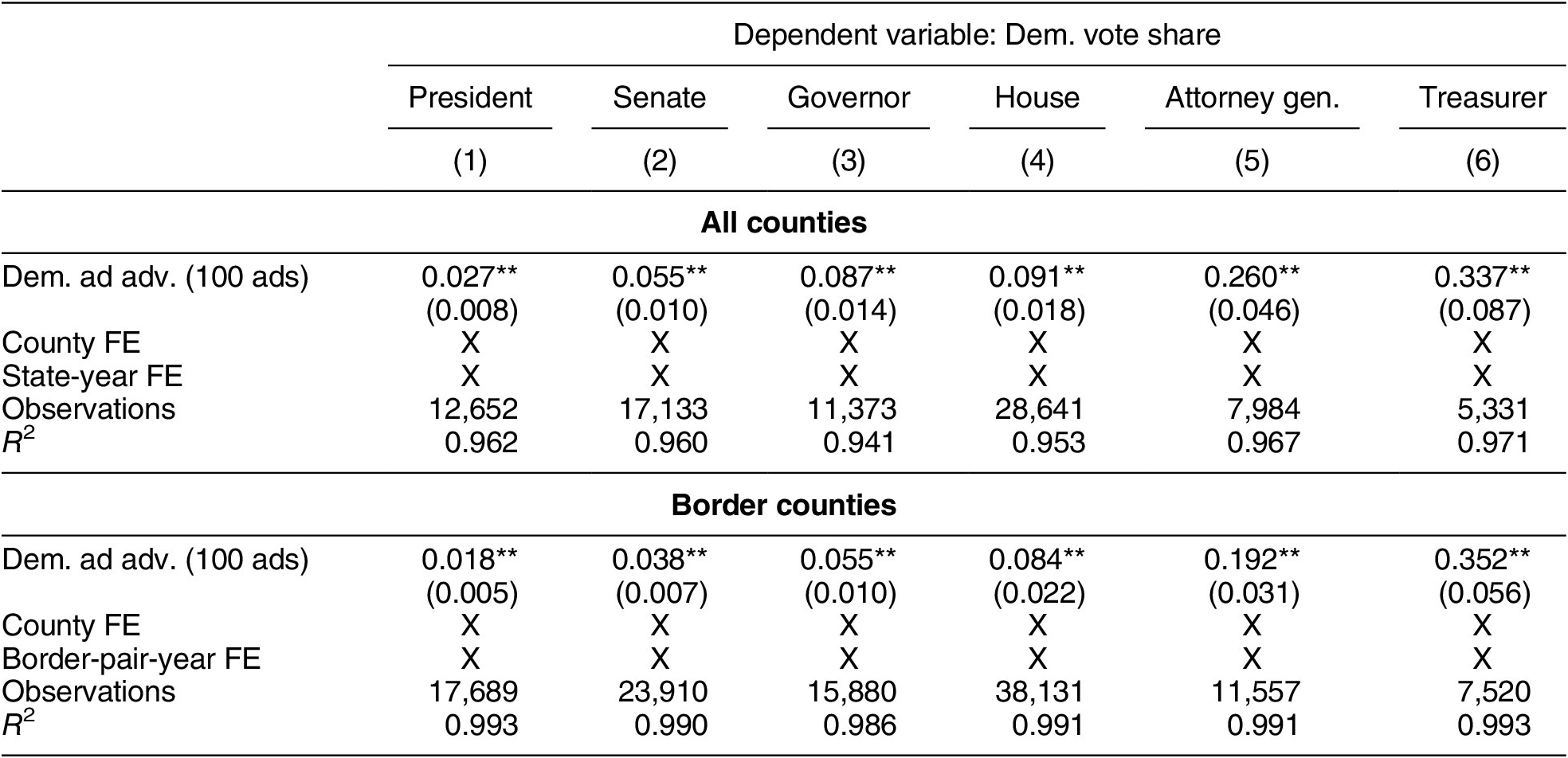
Note: The treatment variable is Democratic ad advantage in terms of hundreds of ads.Standard errors are clustered by county and DMA-year in the top panel and by county and DMA border-year in the bottom panel. *p < 0.05; **p < 0.01.
The results from both designs tell the same story: a similar-sized ad-airing advantage has much larger effect in down-ballot elections than in presidential elections. Column 1 recapitulates the earlier finding that a 100-airing advantage in presidential elections leads to about a 0.02-point increase in two-party vote share. But this advantage leads to a 0.04–0.06-point increase in vote share in Senate elections (column 2), a 0.06–0.09-point increase in gubernatorial elections (column 3), a 0.08–0.09-point increase in House elections (column 4), a 0.19–0.26-point increase in Attorney General elections (column 5), and a 0.34–0.35-point increase in state Treasurer elections (column 6). The effect of a particular ad advantage can be anywhere between 2.5 and 19 times greater in down-ballot races than in presidential races.Footnote 18
Figure 3 shows the results graphically based on the border counties design in Table 3.Footnote 19 Specifically, it shows the effect of variation in each party’s advertising between -3 and +3 within-unit standard deviations of the mean within border pairs. We noted earlier that this effect of advertising was about 0.5 percentage points in presidential races. It is larger down-ballot: about 1 point in Senate races, 1.35 points in governor races, 0.9 points in House races, 1.6 points in Attorney General races, and 1.5 points in Treasurer races.Footnote 20

Figure 3. Effect of Democratic Advertising Advantage on Democratic Vote Share
Note: These graphs show the implied effects of a
 $ \pm $
3-standard-deviation shift in Democratic ad advantage for each office. They are based on the residuals from the border counties models in Table 3. The x-axes are the same across plots to enhance comparability. The sizes of the dots reflect the number of paired county-year observations in the respective x-axis bin.
$ \pm $
3-standard-deviation shift in Democratic ad advantage for each office. They are based on the residuals from the border counties models in Table 3. The x-axes are the same across plots to enhance comparability. The sizes of the dots reflect the number of paired county-year observations in the respective x-axis bin.
Not only does advertising have a larger effect in down-ballot races, but it does so at a lower cost.Footnote 21 For presidential races, we estimate that the cost per vote is about $365, or somewhat more than the $170 per vote estimated by Spenkuch and Toniatti (Reference Spenkuch and Toniatti2018) based on the cost of advertising in the 2008 presidential election. A $10 million advantage in an individual state might gain a candidate 27,000 votes, or enough to tip Nevada, Maine, Michigan, Wisconsin, and New Hampshire in the 2016 election. The cost per vote is much lower in other offices: about $200 in Senate races and $125 in gubernatorial races. This suggests that a very plausible ad advantage of $2 million in a Senate race would gain a candidate about 10,000 votes, which is also enough to tip several races in recent years. In addition, the cost per vote from advertising, especially in down-ballot races, is comparable to that of other campaign activities (Green and Gerber Reference Green and Gerber2019, Table 12-1). This may explain why campaigns continue to spend so much on television advertising.
To be sure, these calculations of advertising effects and the implied cost per vote assume that the marginal returns to advertising are constant—that is, they do not diminish as the number of ads aired in a race increases. Figure 3 suggests that advertising advantage does have a fairly linear relationship with vote share. In Appendix E, we examine this question in more detail and find little apparent evidence of diminishing returns. Only at very high levels of advertising do there appear to be diminishing returns. But even at these high levels, vote share is almost always increasing at the margins, suggesting that candidates are still getting something for their dollar. Moreover, these high levels of advertising rarely translate into an advertising advantage for either candidate because the two sides typically match each other’s advertising. Thus, there is little reason for candidates to cease advertising, especially if their opponent continues to stay on the air.Footnote 22
Mechanisms: Persuasion and Partisan Mobilization
What mechanism best accounts for the fact that the effect of television advertising on election outcomes differs across levels of office? We first provide evidence for the mechanism of persuasion—that is, advertising provides information that helps persuade existing voters to support a particular candidate.
Testing for this mechanism requires measures of voters’ knowledge and perceptions of candidates at multiple levels of office. Although only a few surveys include such measures—and, any relationship between individual-level voter attitudes and advertising is necessarily correlational—the evidence suggests that television advertising provides voters information and shapes their views of candidates. Moreover, these effects are larger in down-ballot races than in presidential races.
Lower Levels of Opinion Formation and Strength in Down-Ballot Races
One expectation is that voters should be less likely to have opinions about down-ballot candidates and, if they do, less likely to have strong opinions. This creates riper conditions for persuasion.
We test this expectation in three sets of surveys that contain identical measures of attitudes toward candidates at various levels of office. Two surveys, the 2000 National Annenberg Election Study (NAES) and the American National Election Study (ANES), include measures of favorability toward presidential, US Senate, and US House candidates using a feeling thermometer. We measure whether voters have an opinion based on whether they were able to rate candidates. We also measure the strength of opinions based on whether respondents gave strongly favorable or unfavorable opinions (0–10 or 90–100 on the feeling thermometer).
A third survey, the Cooperative Congressional Election Study (CCES), asks respondents to place presidential, Senate, and House candidates on a seven-point ideological scale ranging from very liberal to very conservative. Again, because respondents could express no opinion, we can measure their level of information about or familiarity with the candidates. We also capture a rough proxy for the strength of their opinion—here, whether they placed a candidate at one of the endpoints of the scale (1 or 7).
To illustrate the general pattern, we average the results in two ways. First, we average the ANES and CCES surveys across years, although the same patterns do hold within the individual survey years.Footnote 23 Second, we average views of the opposing candidates to create one quantity for each level of office, acknowledging that there can be variation within levels of office depending on the visibility of the individual candidates.
Table 4 presents the percentage of respondents who could not rate or place the candidate and the percentage of respondents who had an “extreme” rating or placement (among those who had an opinion). The findings confirm expectations. First, a much larger percentage of respondents fail to rate House and Senate candidates or place them on this ideological scale, compared with presidential candidates. For example, almost all respondents could rate the presidential candidates on feeling thermometers, but between 20% and 40% could not rate House or Senate candidates. Senate candidates were marginally more familiar than House candidates. It was also much harder for respondents to place House or Senate candidates on ideological scales. Indeed, an average of nearly half (47%) of CCES respondents could not place House candidates.
Table 4. The Existence and Extremity of Views about Presidential, Senate, and US House Candidates

Second, among those who could rate or place the candidates, a larger percentage had extreme views of presidential candidates than Senate or House candidates. In the ANES data, for example, an average of 21% of respondents rated the presidential candidates very unfavorably or very favorably, but 10% or less did this for Senate or House candidates. In the CCES, a smaller fraction placed Senate or House candidates at the endpoints of the ideological scale as well.
To be sure, these results are hardly definitive. Because the surveys are conducted during or after the election campaign in each year, they cannot capture attitudes before exposure to campaign advertising. However, this likely militates against finding information asymmetries across levels of office, especially given the stronger relationship between advertising and voter attitudes about down-ballot candidates, which we report below. Thus, these results still suggest that the persuasive potential of advertising should be larger in down-ballot races.
Larger Effects of Advertising on Views of Down-Ballot Candidates
If advertising helps persuade voters, the other main empirical implication is that it will have larger effects on knowledge about and feelings toward candidates in down-ballot races relative to presidential races. We evaluate this claim in two ways.
First, we evaluate whether advertising helps inform voters about the candidates. For each respondent in the 2006–18 CCES surveys, we calculate the percentage of candidates for each office for whom they provide an ideological placement. We then regress this percentage on the total number of ads at each level of office aired in the month prior to the survey interview. These models also include constituency-year-period fixed effects and control for pretreatment demographic characteristics of respondents (gender, race, education, and age).
We find that ads reduce the percentage of “don’t know” responses at each level of office but do so much more in down-ballot races (Table 5). For every additional 100 ads aired, there is a very modest (and statistically insignificant) decline in the proportion of presidential candidates that the respondents cannot place on this ideological scale. But the same number of ads creates a decline that is about seven times larger in Senate races and 16 times larger in House races. In the ANES data, advertising also reduces the proportion of respondents who cannot rate the candidates on a feeling thermometer and, again, especially in down-ballot races. Advertising appears to increase knowledge to a greater extent in exactly those races where knowledge is less prevalent.
Table 5. The Effects of Advertising on Knowledge of the Candidates

Note: Standard errors clustered by DMA-year. *p < 0.05; **p < 0.01.
Second, we evaluate whether advertising appears to have a larger effect on voters’ attitudes about down-ballot candidates compared with its influence on attitudes about presidential candidates. We operationalize attitudes in terms of both candidates’ valence (likeability, quality, experience, etc.) and their ideological proximity to voters. We examine these two characteristics because they derive from prominent theories of how voters make decisions (e.g., Buttice and Stone Reference Buttice and Stone2012). (To be sure, we are not testing these theories or making claims about their explanatory power.)
We assess valence in the NAES and ANES surveys by subtracting the Republican candidate’s favorability score from the Democrat’s score to produce the Democrat’s valence advantage. We then regress this valence advantage on the Democratic ad advantage in a model that also includes state and year fixed effects and pretreatment demographic characteristics (gender, race, education, and age).Footnote 24
The top panel of Table 6 shows the results from the ANES. A 100-ad advantage has no effect on the Democrats’ valence advantage in the 2000–16 presidential elections but increased valence advantages by much more in Senate elections (0.23) and House elections (0.52). In the NAES, the effect of ads on candidates’ favorability ratings is also larger for down-ballot candidates than for presidential candidates, although the point estimates have larger standard errors due to smaller sample sizes.
Table 6. The Effects of Advertising on Candidate Valence and Ideological Proximity

Note: Standard errors clustered by DMA-year. *p < 0.05; **p < 0.01.
Next, we examine whether advertising affects the ideological proximity between voters and candidates. Using the 2006–2018 CCES surveys, we calculate proximity as the absolute distance between the self-placement of respondents and their placement of candidates on the seven-point ideology scale. We then calculate the ideological advantage of the Democratic candidate as respondents’ ideological congruence with Democratic candidates minus their congruence with Republican candidates. We regress this proximity advantage on the Democratic ad advantage, constituency-year and county fixed effects, and demographic characteristics of respondents (gender, race, education, and age).
The bottom panel of Table 6 shows the results. A 100-ad Democratic advantage in presidential elections is associated with a 0.007 increase in the Democratic candidate’s proximity advantage (p = 0.07). This same ad advantage is associated with a 0.012 shift in Senate elections and a 0.010 shift in House elections (p = 0.20). Although these results are not as clear-cut as the valence results, they also suggest that television advertising can influence perceived spatial proximity to the candidates, and more so in down-ballot races than presidential races.
Partisan Turnout as an Alternative Mechanism
Finally, we examine whether television advertising influences election outcomes by altering the balance of Democrats and Republicans who vote. This mechanism is not consistent with the results thus far, especially the differing effects of ads across levels of office, but it deserves a formal test nonetheless. To conduct a test, we obtained administrative data from state voter files compiled by the firm Catalist. These data contain the percentage of Democrats and Republicans that voted in each county in the elections between 2008 and 2018. This includes the 31 states that record party registration and 18 states where Catalist models partisanship based on demographics and local voting patterns.Footnote 25 We calculate the Democratic Party’s turnout advantage as the difference between the percentage of Democrats that turn out to vote and the percentage of Republicans that turn out. We then model this as a function of the Democratic Party’s overall advertising advantage, summing all advertising across presidential, Senate, governor, House, Attorney General, and Treasurer races. This does not capture every advertisement, as there are a small number of ads for other offices, ballot propositions, and so on, but it does capture the vast majority of ads that could affect partisan turnout. To estimate these models, we use the entire set of counties from these states as well as the relevant border county pairs, just as in our analyses of advertising and election outcomes.
Overall, the results are mixed (Table 7). In the model with all counties, a Democratic ad advantage is associated with a small turnout advantage for Democrats (and vice versa for Republicans), but in the model with border county pairs, there is no relationship. This latter null result is arguably more credible because this model is less vulnerable to time-varying confounders or trends than is the all-counties model. For instance, if one party’s candidates all tend to target more ads to a county that is trending in their direction, this could lead to a spurious finding of advertising effects. But even in the all-counties model, the size of the point estimate (b = 0.015) is small enough that partisan turnout cannot explain advertising’s effect on election outcomes, particularly in down-ballot elections. This is because a small effect of advertising on partisan turnout, combined with the modest relationship of partisan turnout to election outcomes, implies a small total effect on election outcomes (see Appendix F for more details).Footnote 26
Table 7. The Effects of Advertising on Partisan Turnout

Note: Standard errors clustered by county and DMA-year in top panel and county and DMA border-year in bottom panel. *p < 0.05; **p < 0.01.
A second test of whether advertising affects partisan turnout is whether advertising aired to influence one level of office “spills over” and affects outcomes at other levels.Footnote 27 For example, if a Democratic advantage in presidential election advertising increases the Democratic advantage in turnout overall, this should help Democratic candidates down the ballot. We estimate the same county-level models of election outcomes including not only advertising in that race but also advertising in other races. If advertising spills over across races, we would expect that advertising in other offices would affect vote margins.
We do not find consistent spillover at any level of office (Table 8). In the model using all counties, there is evidence of small spillover effect, but the border counties model shows no such effects. This is consistent with the evidence in Table 7.Footnote 28 Taken together, advertising’s effect on election outcomes—and especially its differential effect across levels of office—has more to do with persuasion than the mobilization of partisans.
Table 8. Spillover of Television Advertising across Offices (2000–2018)

Note: Standard errors clustered by county and DMA-year in top panel; county, DMA border-year in bottom. *p < 0.05; **p < 0.01.
Conclusion
Television advertising is the cornerstone of many campaigns for political office in the United States. As scholars have developed more detailed data and sophisticated estimation strategies, they have shown that television advertising is related to election outcomes: the larger a candidate’s advantage in advertising compared with that of their opponent, the larger their share of the vote. The extant literature has demonstrated this in some presidential and US Senate elections. But no study has systematically examined the effect of advertising across levels of office, including different types of down-ballot races.
We have provided the most comprehensive analysis of advertising effects to date. We find that television advertising affects election results across all levels of office but that the effects of advertising are substantially larger in down-ballot elections than presidential elections. Despite increasing partisanship in the electorate, there are still persuadable voters that respond to television advertising—especially in down-ballot elections, where voters have less information about candidates. Of course, this relative difference in advertising’s effect does not mean that its effect is “large” in some absolute sense or large enough to potentially change the outcome of an election. That would be most likely in close races where one party is able to muster a substantial advertising advantage. But we do not claim that this is a common occurrence.
We also provide important evidence for the mechanism that underlies this relationship between advertising and election outcomes. We show that advertising has larger effects in down-ballot races because it provides new information and changes voters’ attitudes about the candidates. We show that voters clearly have less information and weaker opinions about candidates in down-ballot races. We also show that advertising has a stronger relationship with the formation and direction of attitudes about the candidates. In short, advertising appears to persuade voters. We find less evidence for a competing mechanism—that advertising mobilizes partisans to vote.
This evidence about mechanisms is important in at least two ways. For one, it helps clarify how a central form of campaign communication influences voters. Campaigns obviously care about both persuasion and mobilization, albeit to varying degrees. But different campaign tactics can be more or less effective at these different tasks. Our evidence suggests that the primary benefit of television advertising is providing voters with information and shifting their attitudes about the candidate.
Second, evidence about individual-level mechanisms addresses the forces that create over-time changes in aggregate election outcomes. As Hill, Hopkins, and Huber (Reference Hill, Hopkins and Huber2021, 1) note, “Changes in partisan outcomes between consecutive elections must come from changes in the composition of the electorate or changes in the vote choices of consistent voters.” Both of these pathways are important, but in recent elections, including 2012 and 2016, persuasion has been particularly important (Hill, Hopkins, and Huber Reference Hill, Hopkins and Huber2021). Television advertising is thus potentially crucial to explaining both the choices of individual voters and why outcomes shift from election to election.
We are also mindful of the limitations of our analysis. Our findings do not necessarily address the effects of advertising in other media, such as online media. Some evidence suggests that advertising online reflects different strategic goals than persuasion, such as fundraising (Ridout, Fowler, and Franz Reference Ridout, Fowler and Franz2021, 8). It is also the case that current political trends—such as the rise of online electioneering and the decline of split-ticket voting (Jacobson Reference Jacobson2021)—could eventually lead to a decrease in the effect of television advertising on elections. However, we do not yet see evidence that its effect has changed over the 18-year period that we study (see Appendix I).
Our findings also do not address the effects of the specific messages in ads, such as which issues they focus on or whether they primarily support or attack a candidate. Our data and research design are well suited to identifying the effects of advertising volume but not these other characteristics.Footnote 29 Future studies can build on our research to specify what components of ads most help to persuade voters (see, e.g., Gordon et al. Reference Gordon, Lovett, Luo and Reeder2019).
Supplementary Materials
To view supplementary material for this article, please visit http://doi.org/10.1017/S000305542100112X.
Data Availability Statement
Research documentation and most of the data that support the findings of this study are openly available at the American Political Science Review Dataverse: https://doi.org/10.7910/DVN/F8JXHR. As we discussed in the main text in footnotes 4 and 6, some of the elections and advertising data for our analyses are obtained under restricted license. We provide more details in the readme file on the Dataverse about how researchers can obtain and compile these files.
Acknowledgments
We wish to thank the editors and anonymous reviewers for their feedback. We are grateful for feedback from Justin de Benedictis-Kessner, David Broockman, Kevin Collins, Rich Davis, James Mulhall, Robert Erikson, Anthony Fowler, Don Green, Andrew Hall, Ethan Porter, Julian Wamble, Michael Miller, Eitan Hersh, Seth Hill, Dan Hopkins, Josh Kalla, Otis Reid, Aaron Strauss, Travis Ridout, and Daron Shaw. We also appreciate feedback from participants in workshops at George Washington University, Vanderbilt University, Stony Brook University, and the University of Maryland.
Conflict of Interest
The authors declare no ethical issues or conflicts of interest in this research.
Ethical Standards
The authors affirm this research did not involve human subjects.


 Open access