
Abstract
Uncertainty has an almost negligible impact on project value in the standard economic model. I show that a comprehensive evaluation of uncertainty and uncertainty attitude changes this picture fundamentally. The illustration of this result relies on the discount rate, which is the crucial determinant in balancing immediate costs against future benefits, and the single most important determinant of optimal mitigation policies in the integrated assessment of climate change. First, the paper removes an implicit assumption of (intertemporal or intrinsic) risk neutrality from the standard economic model. Second, the paper introduces aversion to non-risk uncertainty (ambiguity). I show a close formal similarity between the model of intertemporal risk aversion, which is a reformulation of the widespread Epstein–Zin–Weil model, and a recent model of smooth ambiguity aversion. I merge the models, achieving a threefold disentanglement between risk aversion, ambiguity aversion, and the propensity to smooth consumption over time.


Notes
Almost all large- scale integrated assessment models deriving optimal policies are based on a representative agent employing the standard economic model. In regional models, like the Nordhaus (2011) RICE model, each regions is represented by such a representative agent.
In the original smooth ambiguity model, aversion to standard or objective risk is set equal to the propensity to smooth consumption over time. Only aversion to subjective risk, or second-order uncertainty, is disentangled from this intertemporal smoothing preference. Thus, the original smooth ambiguity model conflates ambiguity aversion with well-known risk characteristics: objective risk aversion is usually larger than the propensity to smooth consumption intertemporally. Introducing a disentanglement from intertemporal smoothing only for subjective uncertainty results in an unfair comparison between the effects of risk and ambiguity aversion.
They find a coefficient of smooth ambiguity aversion very close to the risk aversion coefficients I discuss in the context of risk aversion. However, their approach exogenously assumes a low value of Arrow–Pratt (and, thus, intertemporal) risk aversion. Then, their coefficient of relative smooth ambiguity aversion picks up the remaining aversion necessary to explain asset prices.
In particular, some ambiguity models (but not the smooth ambiguity model) imply time-inconsistent decisions, which might not be considered rational or normatively desirable.
Formally, \(X\) is a compact metric space and \(p\in P\) an element of the space of Borel probability measures on \(X\).
See Eq. (9) and footnote 22 for a mathematically more explicit statement of this trade-off.
The parameter \({\sigma }\) characterizes risk in the sense of volatility. In the climate change debate, risk is frequently used to also denote a reduction in the expected value, e.g., as a consequence of catastrophic events. Such a reduction mostly affects the expected growth term of the social discount rate.
Moreover, Dasgupta (2008) points out that, from a normative perspective, an egalitarian choice of \(\delta =0.1\,\%\) should also call for a higher propensity of intergenerational consumption smoothing \(\eta >1\).
The growth rate is endogenous in the DICE model and has been reconstructed from Nordhaus (2007, 694).
Kocherlakota (1996) estimates \(\mu =1.8\,\%\) and \({\sigma }=3.6\,\%\) based on 90 years of annual data for the United States.
See Kihlstrom and Mirman (1974) for the complications that arise when trying to extend the Arrow–Pratt risk measures to a multi-commodity setting. Even more interestingly, measures of intertemporal risk aversion can be applied straightforwardly to contexts where impacts do not have a natural cardinal scale.
Note that, in general, preferences represented by Eq. (3) cannot be represented by an evaluation function of the form \(U^s(x_1,p)=u_1(x_1)+ {\hbox {E}}_p u_2(x_2)\).
I abandon pure time preference for the sake of simplicity in the characterization only. This step does not change the intuition of the axiom with respect to its general form. Obviously, I keep pure time preference when discussing discount rates.
The strong notion would involve the additional requirement \((x^*,x_1) \not \sim (x^*,x_2)\) in the premise and a strict preference in the implication.
The lottery on the right-hand side of Eq. (4) will make the decision maker either better off or worse off than \((x^*,x^*)\), whereas, on the left-hand side, the decision maker knows that if he picks an inferior outcome for some period, he certainly receives the superior outcome in the other. Calling preferences satisfying Eq. (4) intertemporal risk averse is motivated by the facts that, first, the definition intrinsically builds on intertemporal trade-offs and, second, Normandin and St-Amour (1998, 268) make the point that the conventional Arrow–Pratt measure of risk aversion is an atemporal concept.
A decision maker is defined as (weakly) intertemporal risk loving if the preference relation \(\succeq \) in Eq. (4) is replaced by \(\preceq \). He is defined to be risk neutral if he is both intertemporal risk loving and intertemporal risk averse (relation \(\succeq \) in Eq. (4) is replaced by \(\sim \)).
In a multi-period framework Eq. (5) translates into the recursion

To obtain the normalization used by Epstein and Zin (1989, 1991), multiply Eq. (\(\star \)) by \((1-\beta )(1-\eta )\) and take both sides to the power of \(\frac{1}{{1-\eta }}\). Define \(U^*(x_{t-1},p_t)=\left( (1-\beta ){1-\eta } U(x_{t-1},p_t)\right) ^{\frac{1}{{1-\eta }}}\). Expressing the resulting transformation of Eq. (\(\star \)) in terms of \(U^*\) delivers their version
$$\begin{aligned} {U}^*(x_{t-1},p_t)= \left( (1-\beta )x_{t-1}^{{1-\eta }} + \beta \left[ {\hbox {E}}_{p_{t}} \left( {U}^*(x_{t},p_{t+1}) \right) ^{1-{{\mathrm{RRA}}}} \right] ^{\frac{{1-\eta }}{1-{{\mathrm{RRA}}}}} \right) ^{\frac{1}{{1-\eta }}}. \end{aligned}$$In the standard model, the Arrow–Pratt measure of relative risk aversion depends on what is considered the \(x=0\) level. For example, whether or not breathing fresh air is part of consumption or whether human capital is part of wealth changes the Arrow–Pratt coefficient.
Note that positivity of \({{\mathrm{RIRA}}}\) indicates intertemporal risk aversion independently of whether \(f\) is increasing and concave or decreasing and convex (see footnote 34). In both cases, \(-\frac{f^{\prime \prime }}{f^{\prime }}\) is positive. Moreover, measuring utility in negative units as in the isoelastic case for \(\rho <0\) makes \( z \) negative. Therefore, the definition of relative risk aversion has to employ the absolute of the variable \( z \) (Traeger 2010a). The same reasoning applies to the measure of smooth ambiguity aversion.
These models have to make assumptions about the covariance of consumption growth and stock returns, the share of stocks in the financial wealth portfolio, the properties of the expected returns to human capital, and the share of human capital in overall wealth.
The Epstein–Zin preference representation in Eq. (5) implies a switch in the sign of utility when \(\eta \) crosses unity. During this sign, switch \(1-\eta \) goes through zero, while \({{\mathrm{RIRA}}}\) has a pole. One could redefine \({{\mathrm{RIRA}}}|1-\eta ^2|\) as the actual measure of intertemporal risk aversion, as it is positive if and only if Eq. (4) holds. I stick to the definition in Eq. (7) because this measure is completely analogous to the measure suggested for smooth ambiguity aversion.
In this case, the formula above reduces to a more precise notation of what is commonly written as \(\frac{\mathrm{d}}{\mathrm{d}x_2} \ldots {\hbox {E}}_{p} \ldots u(x_2) \ \): the above notation makes explicit that (for \(y=1\)) the marginal unit (\(\epsilon \) or \(\mathrm{d}x_2\)) in the decision maker’s trade-off is certain, while the baseline \(x_2\) is uncertain.
Observe that also the first-period derivative in Eq. (9) can be rewritten as \(\frac{\mathrm{d}}{\mathrm{d}\epsilon _1}u(x_1+\epsilon _1 y_1)|_{\epsilon _1=0,y_1=1}\mathrm{d}\epsilon _1\).
Modeling an infinitesimal share of a non-marginal unit project rather than a marginal project itself is important. It is well known that risk effects are second-order effects. Therefore, stochasticity effects of an infinitesimal project would vanish.
Let \(\mu _y\) denote the expected value of (the marginal distribution of) \(\ln y\). The condition \({\hbox {E}}y=1\) implies \(\mu _y=-\frac{\sigma _y^2}{2}\). Making use of this constraint, it is Var\((y)=e^{\sigma _y^2}-1 \approx \sigma _y^2+\frac{\sigma _y^4}{2}\). Thus, in the percentage range, \(\sigma _y\) also approximates well the standard deviation of the project \(y\) itself. I refer to \(\kappa \) as the correlation between the project and the baseline even though, more precisely, it is the correlation between \(\ln y\) and the growth rate \(g=\ln \frac{x_2}{x_1}\).
The entries in Table 1 correspond to the intersections of the corresponding curves on the left of Fig. 3 with the dotted \(45^{\circ }\) line. The shape of the curves for \(\kappa =1\) demonstrates why there is no solution to Eq. (12) (no intersection of the \(\kappa =1\) curves with the dotted line).
Fig. 3 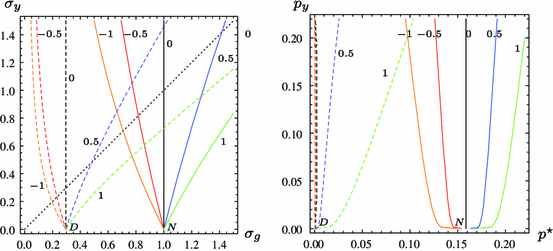
Depicts the combinations of standard deviations (left) and probabilities (right) of baseline growth (horizontal axis) and project payoff (vertical axis) implying a discount rate reduction to the rate of pure time preference. \(p^\star \) represents the probability of being worse off in 50 years than today under a normally distributed growth rate with expected value of \(2\,\%\) per year. \(p_y\) represents the probability that the payoff of the stochastic unit project lies outside of the interval \([0.5,2]\). The numbers labeling the curves denote the correlation \(\kappa \) between baseline growth and project payoff. The dashed curves (originating at “D”) are based on the disentangled approach, and the solid curves (originating at “N”) are based on Nordhaus’ entangled preferences. The intersections of the curves in the left graph with the dotted line (identity) depicts the \(\sigma \) values reported in Table 1
Note that such a translation into probabilities is possible because the marginal distribution of the bivariate normal only depends on the volatility in the remaining dimension. Also note that the vertical range of the right graph corresponds to a \(\sigma _y\)-range of \([0,0.5]\).
In an alternative representation, I could apply the inverse of the function \(f\) characterizing intertemporal risk aversion in front of \(\varPhi ^{-1}\) instead of its current position where it acts on the expected value operator. Then, the same preferences are represented with a different function \(\varPhi \) that would characterize only “access aversion” to ambiguity as opposed intertemporal risk aversion.
Note that Weitzman (2009) puts the prior on the variance \({\sigma }\) rather than on the expected value of growth. He loosely relates the uncertainty to climate sensitivity. The above is a significantly simplified, but insightful, perspective on Weitzman’s approach—abstracting from learning.
Paralleling this paper is a work by Ju and Miao (2012) using a similar model of threefold disentanglement. However, the authors fix Arrow–Pratt risk aversion exogenously to a level significantly lower than in the cited estimates of Vissing-Jørgensen and Attanasio (2003), Bansal and Yaron (2004), and Basal et al. (2010) and then find an ambiguity measure in the range these papers estimate for standard risk aversion.
The numbers represent the risk-free rate calculated in Eq. (8), and the risk-free rate less the term \(h(\cdot )\) evaluated for \(\sigma _g=\sigma _y=0.3236\) corresponding to \(p^\star =0.1\,\%\).
Recasting the proposition for a strictly decreasing continuous function \(f:U\rightarrow {\mathbb R}\) turns concavity in statement (a) into convexity [and convexity into concavity]. Replacing the definition of intertemporal risk aversion by its strict version given in footnote 15 switches concavity to strict concavity in the statement.
Alternatively use \(\sim \) and = instead of \(\succeq \) and \(\ge \) in part (a) and use Aczél (1966, 46).


References
Aczél, J.: Lectures on Functional Equations and Their Applications. Academic Press, New York (1966)
Asheim, G., Mitra, T., Tungodden, B.: Sustainable recursive social welfare functions. Econ. Theory 49(2), 267–292 (2012)
Azfar, O.: Rationalizing hyperbolic discounting. J. Econ. Behav. Organ. 38, 245–252 (1999)
Bansal, R., Kiku, D., Yaron, A.: Long run risks, the macroeconomy, and asset prices. Am. Econ. Rev. Pap. Proc. 100, 542–546 (2010)
Bansal, R., Yaron, A.: Risks for the long run: a potential resolution of asset pricing puzzles. J. Finance 59(4), 1481–1509 (2004)
Campbell, J.Y.: Understanding risk and return. J. Polit. Econ. 104(2), 298–345 (1996)
Chichilnisky, G.: Economic theory and the global environment. Econ. Theory 49(2), 217–225 (2012)
Dasgupta, P.: Commentary: the stern review’s economics of climate change. National Institute Economic Review 2007; 199; 4 (2008)
Dasgupta, P.: Discounting climate change. J. Risk Uncertain. 37, 141–169 (2009)
Dell, M., Jones, B., Olken, B.: Temperature shocks and economic growth: evidence from the last half century. Am. Econ. J. Macroecon. 4(3), 66–95 (2012)
Ellsberg, D.: Risk, ambiguity and the savage axioms. Q. J. Econ. 75, 643–669 (1961)
Epstein, L.G., Zin, S.E.: Substitution, risk aversion, and the temporal behavior of consumption and asset returns: a theoretical framework. Econometrica 57(4), 937–969 (1989)
Epstein, L.G., Zin, S.E.: Substitution, risk aversion, and the temporal behavior of consumption and asset returns: an empirical analysis. J. Polit. Econ. 99(2), 263–286 (1991)
Figuiéres, C., Tidball, M.: Sustainable exploitation of a natural resource: a satisfying use of Chichilnisky’s criterion. Econ. Theory 49(2), 243–265 (2012)
Ghirardato, P., Maccheroni, F., Marinacci, M.: Differentiating ambiguity and ambiguity attitude. J. Econ. Theory 118(2), 122–173 (2004)
Gierlinger, J. Gollier, C.: Socially efficient discounting under ambiguity aversion. IDEI Working Papers 561, Institut d’Économie Industrielle (IDEI), Toulouse (2008)
Gilboa, I., Schmeidler, D.: Maxmin expected utility with non-unique prior. J. Math. Econ. 18(2), 141–153 (1989)
Gollier, C.: Discounting an uncertain future. J. Public Econ. 85, 149–166 (2002)
Hansen, L.P., Sargent, T.J.: Robust control and model uncertainty. Am. Econ. Rev. 91(2), 60–66 (2001)
Hardy, G., Littlewood, J. Polya, G.: Inequalities, 2 edn, Cambridge University Press. First published 1934 (1964)
Heal, G.: Climate economics: a meta-review and some suggestions for future research. Rev. Environ. Econ. Policy 3(1), 4–21 (2009)
Heutel, G.: How should environmental policy respond to business cycles? Optimal policy under persistent productivity shocks. University of North Carolina, Greensboro, Department of Economics working paper series vol. 11, no. 08 (2011)
Hoel, M., Karp, L.: Taxes and quotas for a stock pollutant with multiplicative uncertainty. J. Public Econ. 82(1), 91–114 (2001)
Hoel, M., Karp, L.: Taxes and quotas for a stock pollutant. Resour. Energy Econ. 24, 367–384 (2002)
Horowitz, J., Lange, A.: What’s wrong with infinity—a note on Weitzman’s dismal theorem. Working paper (2009)
Ju, N., Miao, J.: Ambiguity, learning, and asset returns. Econometrica 80(2), 559–591 (2012)
Karp, L.: Global warming and hyperbolic discounting. J. Public Econ. 89, 261–282 (2005)
Karp, L., Zhang, J.: Regulation with anticipated learning about environmental damages. J. Environ. Econ. Manag. 51, 259–270 (2006)
Karp, L., Zhang, J.: Taxes versus quantities for a stock pollutant with endogenous abatement costs and asymmetric information. Econ. Theory 49(2), 371–409 (2012)
Keller, K., Bolkerand, B.M., Bradford, D.F.: Uncertain climate thresholds and optimal economic growth. J. Environ. Econ. Manag. 48, 723–741 (2004)
Kelly, D., Kolstad, C.D.: Malthus and climate change: betting on a stable population. J. Environ. Econ. Manag. 41(1), 135–161 (2001)
Kelly, D.L.: Price and quantity regulation in general equilibrium. J. Econ. Theory 125(1), 36–60 (2005)
Kihlstrom, R.E., Mirman, L.J.: Risk aversion with many commodities. J. Econ. Theory 8(3), 361–388 (1974)
Klibanoff, P., Marinacci, M., Mukerji, S.: A smooth model of decision making under ambiguity. Econometrica 73(6), 1849–1892 (2005)
Klibanoff, P., Marinacci, M., Mukerji, S.: Recursive smooth ambiguity preferences. J. Econ. Theory 144, 930–976 (2009)
Kocherlakota, N.R.: The equity premium: it’s still a puzzle. J. Econ. Lit. 34, 42–71 (1996)
Kreps, D.M., Porteus, E.L.: Temporal resolution of uncertainty and dynamic choice theory. Econometrica 46(1), 185–200 (1978)
Lauwers, L.: Intergenerational equity, efficiency, and constructibility. Econ. Theory 49(2), 227–242 (2012)
Leland, H.E.: Saving and uncertainty: the precautionary demand for saving. Q. J. Econ. 82(3), 465–473 (1968)
Lind, R. (ed.): Discounting for Time and Risk in Energy Policy. Resources for the Future, Washington, D.C (1982)
Lucas, R.E.: Models of Business Cycles. Blackwell, New York (1987)
Maccheroni, F., Marinacci, M., Rustichini, A.: Ambiguity aversion, robustness, and the variational representation of preferences. Econometrica 74(6), 1447–1498 (2006a)
Maccheroni, F., Marinacci, M., Rustichini, A.: Dynamic variational preferences. J. Econ. Theory 128(1), 4–44 (2006b)
Millner, A.: On welfare frameworks and catastrophic climate risks. Working paper (2011)
Newell, R.G., Pizer, W.A.: Regulating stock externalities under uncertainty. J. Environ. Econ. Manag. 45(2, Supplement), 416–432 (2003)
Nordhaus, W.D.: A review of the Stern review on the economics of climate change. J. Econ. Lit. 45(3), 686–702 (2007)
Nordhaus, W.D.: A Question of Balance: Economic Modeling of Global Warming, Yale University Press, New Haven. Online preprint: A Question of Balance: Weighing the Options on Global Warming Policies (2008)
Nordhaus, W.D.: An analysis of the dismal theorem. Cowles Foundation discussion paper (1686) (2009)
Nordhaus, W. D.: Estimates of the social cost of carbon: Background and results from the rice-2011 model. NBER working papers 17540, National Bureau of Economic Research (2011)
Nordhaus, W.D.: Economic policy in the face of severe tail events. J. Public Econ. Theory 14(2), 197–219 (2012)
Normandin, M., St-Amour, P.: Substitution, risk aversion, taste shocks and equity premia. J. Appl. Econom. 13(3), 265–281 (1998)
Pindyck, R.S.: Uncertain outcomes and climate change policy. Working paper 15259 (2009)
Pindyck, R.S.: Modeling the impact of warming in climate change economics. In: Libecap, G.D., Steckel, R.H. (eds.) The Economics of Climate Change: Adaptations Past and Present. University of Chicago Press, Chicago (2011)
Plambeck, E.L., Hope, C., Anderson, J.: The Page95 model: integrating the science and economics of global warming. Energy Econ. 19, 77–101 (1997)
Ramsey, F.P.: A mathematical theory of saving. Econ. J. 38(152), 543–559 (1928)
Rezai, A., Foley, D., Taylor, L.: Global warming and economic externalities. Econ. Theory 49(2), 329–351 (2012)
Selden, L.: A new representation of preferences over ‘cerain\(\times \)uncertain’ consumption pairs: the ‘ordinal certainty equivalent’ hypothesis. Econometrica 46(5), 1045–1060 (1978)
Stern, N. (ed.): The Economics of Climate Change: The Stern Review. Cambridge University Press, Cambridge (2007)
Traeger, C.P.: Intertemporal risk aversion. CUDARE working paper 1102 (2010a)
Traeger, C.P.: Subjective risk, confidence, and ambiguity. CUDARE working paper 1103 (2010b)
Traeger, C.P.: Discounting and confidence. CUDARE working paper 1117 (2011)
Traeger, C.P.: Once upon a time preference—how rationality and risk aversion change the rationale for discounting. CESifo working paper no. 3793 (2012)
Vissing-Jørgensen, A., Attanasio, O.P.: Stock-market participation, Intertemporal substitution, and risk-aversion. Am. Econ. Rev. 93(2), 383–391 (2003)
von Neumann, J., Morgenstern, O.: Theory of Games and Economic Behaviour. Princeton University Press, Princeton (1944)
Weil, P.: Nonexpected utility in macroeconomics. Q. J. Econ. 105(1), 29–42 (1990)
Weitzman, M.: A review of the Stern review on the economics of climate change. J. Econ. Lit. 45(3), 703–724 (2007)
Weitzman, M.: Additive damages, fat-tailed climate dynamics, and uncertain discounting. Economics E-Journal 3 (2009)
Weitzman, M.L.: Why the far-distant future should be discounted at its lowest possible rate. J. Environ. Econ. Manag. 36, 201–208 (1998)
Author information
Authors and Affiliations
Corresponding author
Additional information
I am grateful to Larry Karp, David Anthoff, Christian Gollier, Rick van der Ploeg, Geir Asheim, Svenn Jensen, and to participants of the EAERE 2009, the EEA 2009, and of workshops in Oslo and Santa Barbara in 2010.
Appendices
Appendix 1
Notation: The calculations in the appendix make frequent use of the abbreviations \(\rho =1-\eta \) and \(\alpha =1-{{\mathrm{RRA}}}\), characterizing the exponents of the isoelastic aggregators.
Proof of Proposition 1
The first part of the proof calculates the marginal value of an additional certain unit of consumption in the second period (\(\mathrm{d}x_2\)), expressed in terms of marginal first-period consumption units (\(\mathrm{d}x_1\)). This value derives from the marginal trade-off that leaves aggregate welfare
unchanged:
The second part of the proof translates the relation into rates by defining the social discount rate \(r=-\ln \frac{\mathrm{d}x_1}{-\mathrm{d}x_2}\,\left( =-\ln \frac{\mathrm{d}x_2}{-\mathrm{d}x_1}|_{\bar{U}}\right) \), the rate of pure time preference \(\delta =-\ln \beta \), and \(\eta =1-\rho \,\left( =\frac{1}{\sigma }\right) \). Further below, I make use of the relation \(1=\frac{1-\eta }{\rho }\).
\(\square \)
Proof of Proposition 2
For the isoelastic specification and with the definition,
Eq. (9) translates into
In order to calculate \(\left. \frac{\mathrm{d}}{\mathrm{d}\epsilon } U_2(\epsilon ) \right| _{\epsilon =0}\mathrm{d}\epsilon \) the following definition is useful.
Then,
where equality between the first and the second lines follow from Lebesgue’s dominated convergence theorem. Analogously to step 1 in the proof of Proposition 1, I calculate with \(z=\ln y\)
Similarly,
so that
Substituting the result into Eq. (18) and solving for the discount rate yields
The first line corresponds to Eq. (16) and, thus, Eq. (17), yielding the risk-free discount rate under intertemporal risk aversion. Moreover, the random variable \(y\) was assumed to yield an expected value (project payoff) of unity, which implies
eliminating the last bracket. Finally, \(1-\alpha \) has to be expressed in terms of \(\eta \) (capturing the effects of the standard model) and \({{\mathrm{RIRA}}}\) (capturing the additional effects of intertemporal risk averison). I find for \(\rho >0\) that
and for \(\rho <0\) that
In both cases, this yields
which gives rise to the form stated in the proposition.
Proof of Corollary 1
In case 1 of the risk-free discount rate, Eq. (8) translates \(r_{50} = 50 \delta \) into the condition \(\eta \, 50\mu \mathop {=}\limits ^{!} \eta ^2 \frac{\sigma ^2}{2} + {{\mathrm{RIRA}}}\, |1-\eta ^2| \frac{\sigma ^2}{2}\), which results in the stated equation for \(\sigma \). Similarly in case 2, Eq. (10), \(\sigma =\sigma _g=\sigma _y\), and \(\eta \, 50\mu _g \mathop {=}\limits ^{!} \eta ^2 \frac{\sigma _g^2}{2} + {{\mathrm{RIRA}}}\, |1-\eta ^2| \frac{\sigma _g^2}{2}- \eta \kappa \ \sigma _g \sigma _y - |1-\eta | {{\mathrm{RIRA}}}\kappa \ \sigma _g \sigma _y\) yield the result. Without the condition \(\sigma =\sigma _g=\sigma _y\), the same reasoning gives statement 3 of the corollary.
Proof of Proposition 3
Define for the isoelastic specification
I have to solve once more the equation
for \(r=\ln \frac{\mathrm{d}\epsilon }{-\mathrm{d}x_1}\). Making once more use of the definition
where \(\theta \) replaces \(\mu _g\) in \(p_{(x,y)}\) of Eqs. (19) and (21), I find
With the help of Eq. (22), the expression \(\{ \cdot \}\) calculates to
Acknowledging the equality of Eqs. (20) and (23) and their similarity to the second integrand in Eq. (26) (for \(\rho \leftrightarrow \rho \varphi \)), this second integral becomes
Substituting these results back into Eq. (26) delivers
Substituting this result into Eq. (25) and solving for \(r=\ln \frac{\mathrm{d}\epsilon }{-\mathrm{d}x_1}\) yields analogously to the proof of Proposition 2, the discount rate
The last term can be rearranged to the form
completing the proof. \(\square \)
Proof of Proposition 4
Up to Eq. (26), the proof is identical to that of Proposition 3. In the next step, in \(V_0(\alpha ,0)^{\frac{\rho \varphi }{\alpha }}\) the ambiguity parameter \(\theta \) replaces \(\kappa \) instead of \(\mu _g\). Thus, the first integral in Eq. (26) becomes
For the integrand of the second integral in Eq. (26), I find
delivering the integral
Substituting these results back into Eq. (26) returns the second-period welfare change in \(\epsilon \):
Substituting this result into Eq. (25) and solving for \(r=\ln \frac{\mathrm{d}\epsilon }{-\mathrm{d}x_1}\) yields analogously to the proof of Proposition 2, the discount rate
By symmetry of the hyperbolic sine, the sign of \((\alpha -1)\) can be flipped simultaneously in the numerator and the denominator. Using Eq. (24) to substitute for \((1-\alpha )\) then yields the result stated in the proposition. \(\square \)
Appendix 2
The following proposition formalizes how intertemporal risk aversion, defined in the sense of Eq. (4), translates into the curvature of the function \(f\) in a preference representation of the form (3).Footnote 34
Proposition 5
Let preferences over \(X\times P\) be represented by Eq. (3) with a continuous function \(u:X\rightarrow {\mathbb R}\) and a strictly increasing and continuous function \(f:U\rightarrow {\mathbb R}\), where \(U=u(X)\) and \(\beta =1\).
-
(a)
The corresponding decision maker is (weakly) intertemporal risk averse [loving], if and only if the function \(f\) is concave [convex].
-
(b)
The corresponding decision maker is intertemporal risk neutral, if and only if there exist \(a,b \in {\mathbb R}\) such that \(f(z)=a z + b\). An intertemporal risk neutral decision maker maximizes intertemporally additive expected utility (Eq. (1)).
Proof of Proposition 5
(a) Sufficiency of axiom (4): The premise of axiom (4) translates with \(\beta =1\) into the representation (3) as
Writing the implication of the axiom in terms of representation (3) yields
Combining Eqs. (27) and (28) returns
which for an increasing [decreasing] version of \(f\) is equivalent to
Defining \(z_i=u(x_i)\), the equation becomes
Because preferences are assumed to be representable in the form (3), there exists a certainty equivalent \(x^*\) to all lotteries \(\frac{1}{2} x_1 + \frac{1}{2} x_2\) with \(x_1,x_2 \in X\). Taking \(x^*\) to be the certainty equivalent, the premise and, thus, Eq. (30) have to hold for all \(z_1,z_2 \in u(X)\). Therefore, \(f\) has to be concave [convex] on \(U(x)\) ((Hardy et al. 1964, 75)).
Necessity of axiom 4 The necessity is seen to hold by going backward through the proof of sufficiency above. Strict concavity [convexity] of \(f\) with \(f\) increasing [decreasing] implies that Eq. (30) and, thus, Eq. (29) have to hold for \(z_1,z_2 \in u(X)\). The premise corresponding to (27) guarantees that Eq. (29) implies Eq. (28) which yields the implication in condition (4). Replacing \(\succeq \) by \(\preceq \) and \(\ge \) by \(\le \) in the proof above implies that the decision maker is intertemporal risk averse, if and only if \(f\) is convex [for an increasing version of \(f\) and concave for \(f\) decreasing].
(b) The decision maker is intertemporal risk neutral, if and only if \(f\) is concave and convex on \(u(X)\), which is equivalent to \(f\) being linear.Footnote 35 However, a linear function \(f\) cancels out in representation (3) and makes it identical to the intertemporally additive expected utility standard representation (1).
Appendix 3
1.1 Relation to Proposition 1 and Gollier (2002)
Equation (14) in Gollier (2002) is
where \(\delta =\frac{1}{\beta }-1,\,\tilde{g}=\frac{\tilde{x}_2}{x_1}-1\), and \(\beta \) denotes Gollier’s utility discount factor. The tilde (\(\tilde{}\)) marks random variables. In contrast, Eq. (16) for the isoelastic normal case translates into
Thus, Gollier’s approximate formula underestimates the social discount rate by the term \(\eta \frac{\sigma ^2}{2}\). Much of the difference can be traced back to the first step of his derivation, where the Arrow–Pratt approximation of the certainty equivalent (or equivalently the certainty-equivalent growth rate) loses a term proportional to \(\frac{\sigma ^2}{2}\) in a setting with isoelastic preferences and a normal growth rate.
In a setting with CARA utility and a normal distribution of the growth rate Gollier’s approximation does better. I assume that Gollier’s growth rate \(\tilde{g}=\frac{\tilde{x}_2}{x_1}-1\sim N(\mu ,\sigma ^2)\), which is equivalent to a distribution of second-period consumption \(\tilde{x}_2 \sim N\big (x_1(1+\mu ),x_1^2\sigma ^2\big ) \equiv N(\mu _x,\sigma _x^2)\). Moreover, the assumption of CARA aggregators translates into \(u(x)=-\frac{\exp (-A_u x)}{A_u}\) for utility and \(v(x)=-\frac{\exp (-A_v x)}{A_v}\) for Arrow–Pratt risk aversion, adopting Gollier’s notation where \(A_u\) is absolute aversion to intertemporal substitution and \(A_v\) is absolute aversion to risk in the Arrow–Pratt sense. Then, the resulting exact discount rate becomes
The second line is equivalent to Gollier’s equation (12), before replacing his absolute aversion measures with relative aversion measures. Thus, in the CARA-normal case, the quality of his approximation is given by the quality of the approximation going from Eqs. (31) to (32). For this approximation to hold, risk has to be moderate and expected absolute growth has to be small. Small absolute growth is equivalent to a low expected growth rate or a low present consumption level.
Rights and permissions
About this article
Cite this article
Traeger, C.P. Why uncertainty matters: discounting under intertemporal risk aversion and ambiguity. Econ Theory 56, 627–664 (2014). https://doi.org/10.1007/s00199-014-0800-8
Received:
Accepted:
Published:
Issue Date:
DOI: https://doi.org/10.1007/s00199-014-0800-8
Keywords
- Climate change
- Discounting
- Risk aversion
- Ambiguity
- Cost-benefit analysis
- Intertemporal substitutability
- Uncertainty