
Executive summary
Groundwater monitoring is recommended as a higher-tier option in the regulatory groundwater assessment of plant protection products in the European Union. However, to date little guidance has been provided on study designs. SETAC EMAG-Pest GW, a group of regulatory, academic, and industry scientists, was created in 2015 to establish scientific recommendations for conducting such studies. This report provides the SETAC EMAG-Pest GW group’s recommendations on study designs and study procedures. Because of the need to assess the vulnerability to leaching in both site selection and in extrapolating study results, information on how to assess the vulnerability to leaching is a major topic in this report.
In the development of groundwater study designs, which groundwater needs to be protected and to what level are key aspects. In the European Union, a groundwater quality standard of 0.1 µg/L applies to active substances and relevant metabolites, but the groundwater to which this standard is applied varies among the Member States. Also, the definition of the concentration may consider temporal or spatial variability (e.g. a single sample or an average concentration over a period of time or geographic area). The SETAC EMAG-Pest GW group does not endorse any specific exposure assessment option. However, 7 different exposure assessment options that consider only the location of the groundwater to which the ground water quality standard is applied were selected to illustrate the impact of the exposure assessment option on the study design.
Monitoring can be performed on many different geographical scales. In-field and edge-of-field monitoring focus on residues from applications to a single field, while catchment and aquifer monitoring focus on residues in groundwater over a larger area.
The timing of applications in monitoring studies can vary. In a prospective study, an application is made and the movement and degradation of the residues is followed. In a retrospective study, residues from previous applications are monitored. Some studies are both retrospective and prospective—residues from previous applications are monitored and a new application is made and the residues are followed.
In addition to the exposure assessment option, study designs must consider the objectives of the study, the properties of the active substance and its metabolites, and the site characteristics. Usually, the objective is to determine whether a substance can move into the groundwater specified in the exposure assessment option as well as the magnitude of residues in groundwater. The objective may also include determining degradation rates in soil as a function of depth, persistence and movement of residues in groundwater, efficacy of mitigation measures, or confirmation of more detailed studies on a wider range of sites. Sampling schedules should consider the expected time required for an active substance to move through the soil into groundwater, as well as expected persistence in both soil and groundwater. Movement and persistence can be affected by both site characteristics and properties of the active substance and its metabolites. The need to tailor study designs to objectives, exposure assessment options, compound properties and site characteristics complicates the development of standardised study designs. Therefore, this report includes a number of example designs.
Other key points that must be addressed by study designs are the vulnerability of the chosen sites compared to the vulnerability of all use areas supported by the study, the product use before and during the study, and the connectivity of the sampled groundwater to treated fields. Demonstrating connectivity (a quality criterion in the EU assessment of monitoring sites to exclude false negative measurements) is more challenging for catchment or aquifer monitoring compared to shallow wells installed as part of in-field or edge-of-field studies.
This report includes an extensive discussion on assessing vulnerability of monitoring sites. This includes information on different approaches to vulnerability assessment and mapping as well as for setting monitoring sites into context. Lists of available methods and data sources available at the European level are also included.
In addition to information on study design and estimating vulnerability, this report includes information on a number of other topics: avoiding contamination during sampling and/or analysis, avoiding influencing residue movement as a result of purging during sampling, and proper study documentation (Good Laboratory Practices and/or quality criteria). Procedures that are discussed include site selection (new or existing wells), installation of monitoring wells, sample collection, and analysis of samples. The report also provides information on causes of outliers (abnormally high concentrations not the result of normal leaching through soil), the use of public monitoring data, information on further hydrological characterisation (such as use of tracers, groundwater age dating, and geophysical methods), and information that should be included in reports providing results of groundwater studies.
Abstract
Groundwater monitoring is recommended as a higher-tier option in the regulatory groundwater assessment of crop protection products in the European Union. However, to date little guidance has been provided on the study designs. The SETAC EMAG-Pest GW group (a mixture of regulatory, academic, and industry scientists) was created in 2015 to establish scientific recommendations for conducting such studies. This report provides recommendations for study designs and study procedures made by the Society of Environmental Toxicology and Chemistry (SETAC) Environmental Monitoring Advisory Group on Pesticides (EMAG-Pest). Because of the need to assess the vulnerability to leaching in both site selection and extrapolating study results, information on assessing vulnerability to leaching is also a major topic in this report. The design of groundwater monitoring studies must consider to which groundwater the groundwater quality standard is applicable and the associated spatial and temporal aspects of its application, the objective of the study, the properties of the active substance and its metabolites, and site characteristics. This limits the applicability of standardised study designs. The effect of the choice of groundwater to which the water quality guideline is applied on study design is illustrated and examples of actual study designs are presented.
1 Introduction
In the European Union, placing a plant protection product on the market is regulated by Regulation (EC) No. 1107/2009 and its associated implementing Regulations (i.e., 546/2011 on uniform principles, plus 283/2013 and 284/2013 on data requirements). Regulation 284/2013 requires estimating the concentration of the active substances and their metabolites in groundwater (PECgw), identified as part of the residue definition for risk assessment with respect to groundwater. To estimate the PECgw according to Regulation 284/2013, Annex 9.2.4.1, “relevant EU groundwater models shall be run” by using the ‘Forum for the Co-ordination of pesticide fate models and their Use’ (FOCUS) groundwater guidance document as recommended in the Commission Communication 2013/C 95/02.
The decision-making in the uniform principles (Regulation 546/2011, Annex C 2.5.1.2, corrected by Regulation 2018/676) states that “no authorisation of a Plant Protection Product (PPP) should be granted if the concentration of the active substance or of relevant metabolites, degradation or reaction products in groundwater, may be expected to exceed the lower of (i) the maximum permissible concentration laid down by Directive 2006/118/EC Council Directive 98/83/EC or (ii) the maximum concentration laid down when approving the active substance with Regulation (EC) No 1107/2009 or the concentration corresponding to one tenth of the ADI laid down when the active substance was approved in accordance with Regulation (EC) No 1107/2009, unless it is scientifically demonstrated that under relevant field conditions the lower concentration is not exceeded”. In the vast majority of the cases, provision (i) applies, so the maximum permissible concentration (or groundwater quality standard or parametric value) is 0.1 μg/L (0.5 μg/L for the sum of active substances). It is highlighted that the two parametric values set for “pesticides” and “total pesticides” in Council Directive 98/83/EC are identical to the “groundwater quality standards” values set in Council Directive 2006/118/EC.
Monitoring is useful for determining if groundwater is protected adequately against leaching of active substances and their metabolites (biotic or abiotic degradation products) under relevant field conditions. It is considered as the highest tier in the FOCUS groundwater assessment scheme for assessing potential impacts of active substances and their metabolites (FOCUS 2009; European Commission 2014) (Fig. 1). However, the EFSA PPR Panel criticised the guidance and quality criteria in the FOCUS Tier 4 as too imprecise and the knowledge on groundwater hydrology at the European level as insufficient to demonstrate a safe use at EU level (EFSA 2013).

This document intends to provide scientific recommendations for the conduct of groundwater monitoring and will focus on the conduct of groundwater monitoring studies rather than field leaching studies (Tier 4 as opposed to Tier 3c), although both types of studies can be used to address potential groundwater concerns in the EU registration process (FOCUS 2009; European Commission 2014). The distinction between groundwater monitoring studies and field leaching studies is not always clear, particularly for in-field monitoring studies. However, field leaching studies are usually conducted as a research study with carefully controlled agricultural operations including application of the active substance under supervision of the researcher, while monitoring studies are usually conducted in commercial fields where agricultural operations are managed by the grower. Groundwater monitoring studies typically have less activity per site than field leaching studies, but the work is conducted at more sites, which allows obtaining information over a wide range of use conditions and hydrogeological settings. In this report, a field leaching study always includes measurements in groundwater, but sometimes also includes studies with measurements only in the unsaturated zone (such as lysimeter studies). Also, in some areas public monitoring studies are available, which are usually not targeted towards specific active substances or their metabolites. Those results can be useful to understand the potential of specific active substances and their metabolites to appear in groundwater, when used in the sampled area.
This report focuses on groundwater studies conducted under the EU regulatory framework. However, the technical discussion on study design and conduct is also largely applicable to groundwater studies that are conducted outside the EU.
Groundwater monitoring data for active substances and their metabolites can be categorised in:
-
samples collected from wells installed within treated fields,
-
samples at the edge of treated fields,
-
samples collected within catchments (recharge area for a single well),
-
samples focused on aquifers (defined bodies of groundwater).
All of these types of samples can be useful to assess the potential impact of active substances and their metabolites on groundwater.
One key aspect in developing groundwater study designs is the definition of both groundwater and what groundwater needs to be protected. There is no universally agreed definition for groundwater, although two definitions are “water in any zone of saturation below the soil surface” or “water in the zone of saturation below the permanent water table”. Probably the first definition is the most commonly accepted, yet water in small zones of saturation above the water table is rarely considered as groundwater. For example, under the first definition water perched above less permeable layers would be considered as groundwater. Given this ambiguity, the definition of what can be allowed in water below the soil surface is critical for interpreting the acceptability of active substances and metabolites in groundwater. This definition is commonly referred to as a protection goal. For work to support registration in the EU, the most appropriate definition of groundwater is the definition provided in Article 2 of Directive 200/60/EC which is “all water which is below the surface of the ground in the saturation zone and in direct contact with the ground or subsoil”, which implies that temporary zones of perched water are not included.
The protection goal adopted by the EU Parliament in Regulation (EC) No 1107/2009 and decision-making of the uniform principles in Regulation 546/2011 (Annex C 2.5.1.2, see above), is explicit regarding the maximum permissible concentration and how it relates to risk assessment. While the spatial or temporal scales associated with determining these concentrations are not explicitly specified, they are implicit assumptions in the tools which are required to be used for risk assessment.
In the current groundwater risk assessment in the EU (modelling studies in Tier 1, Tier 2a, Tier 2b, Tier 3a, Tier 3b, and Tier 3d and lysimeter studies in Tier 3c), assessments consist of evaluating movement of active substances and their metabolites in unsaturated zones below 1 m from the soil surface (Fig. 1). This harmonised approach is accepted by the Member States as being precautionary protective for the saturated groundwater zone for large areas and over long time periods. The protection goal implicit in the FOCUS groundwater modelling for EU registration is an overall vulnerability at the 90th percentile considering both spatial and temporal vulnerability for the yearly average concentration in groundwater, located at least one metre below the ground surface. This was obtained by selecting scenarios in nine major agricultural areas in the EU, representative of a range of climatic and soil conditions. Soils representing an 80th percentile vulnerability were selected by expert judgment. The temporal variability was incorporated by performing simulations over a 20 year period (weather data from 1971 to 1997) and estimating potential concentrations in groundwater by considering the total amount of the active substance or metabolite moving past 1 m in the soil during 1 year, dissolved in the total amount of water moving past 1 m during the same year for each of the 20 years. The 80th percentile of the yearly values were compared with the relevant guideline concentrations for active substances and metabolites.
The uniform principles in Regulation 546/2011 (Annex C 2.5.1.2), implicitly considered as the protection goal, allow modelled groundwater concentrations in excess of the guideline to be discarded if “it is scientifically demonstrated that under relevant field conditions the lower concentration is not exceeded”. In the context of plant protection product authorisation in the EU according to Regulation (EC) 1107/2009, one can interpret that groundwater monitoring data would generally be acceptable for risk assessment evaluations, if they are scientifically derived and evaluated.
The FOCUS Tier 4, and sometimes field leaching and lysimeter studies in Tier 3c, intend to demonstrate that under relevant field conditions the groundwater quality standards are not exceeded so there is no risk to groundwater from the leaching of active substances and/or metabolites. However, FOCUS Tier 4 and field leaching studies use measured results from the environmental compartment itself (the saturated groundwater zone), which needs to be protected. Therefore, a specific protection goal for groundwater monitoring data needs to be more precisely defined in depth, time and space, with the same objective as in the lower tier risk assessment to be protective for groundwater over large areas and over long time periods. As a consequence, different specific protection goals may be used among the Member States when evaluating monitoring data compared to lower tier assessments. Since most Member States do not have clearly defined protection goals, it is often unclear what groundwater is subject to the water quality standard. For example, some Member States consider all groundwater (regardless of depth) as subject to the 0.1 µg/L concentration limit. Others consider only groundwater below 1 m from the soil surface as subject to the 0.1 µg/L concentration limit. The Netherlands considers only groundwater located at least 10 m below the soil surface as subject to the 0.1 µg/L concentration limit (LNV 2007). Transient zones of saturation (such as perched water) above the water table may be considered as groundwater by some Member States. Sometimes spatially or temporally averaged concentrations are considered, while other times a single value in time or space is considered. Other examples of protection goals, not in the context of plant protection product authorisation and groundwater risk assessment but for identifying problematic areas with need for action, are the Water Framework Directive (2000/60/EC) and Groundwater Directive (2006/118/EC). Both provide procedures for assessing the chemical status of groundwater, including the consideration of large groundwater bodies. Neither considers the depth of the groundwater for their procedures.
In some cases, monitoring is conducted to determine actual concentrations of non-relevant metabolites in groundwater that are identified by the protection goal adopted by a Member State. A relevance assessment procedure in combination with a limit value of 10 µg/L for non-relevant metabolites in groundwater is defined in the ‘Guidance document on the assessment of the relevance of metabolites in groundwater of substances regulated under Council Directive 91/414/EEC’ (SANCO 221/2000). However, as this document is not legally binding, some Member states apply other limit concentration values for non-relevant metabolites in groundwater under Regulation (EC) 1107/2009. Because groundwater resources are also regulated in terms of drinking water resources, acceptable limit value concentrations can also be different in national drinking water statutes.
Over the past few years, registrants have been conducting monitoring studies with currently registered active substances and their metabolites with an increasing frequency. The aim has been to demonstrate compliance with groundwater standards under actual use conditions in order to maintain registrations, in contrast to the predictions of modelling. Because of the significant resources required for these large scale monitoring programmes, clarity on study designs is needed by both registrants and regulatory authorities. The possibility of measuring concentrations above permissible limits (due to properties of the active substance or metabolite, experimental conditions, or study deficiencies) can never be excluded. However, the risk that a study is rejected due to its design can be avoided with the development of study guidelines. To help develop scientific principles that support such guidelines, SETAC initiated the SETAC EMAG-Pest GW group.
Groundwater monitoring was also one of the major topics discussed at the 7th EU Modelling Workshop held in Vienna on 21 to 23 October 2014, a meeting of regulatory, industry, and academic scientists. The discussions that took place on groundwater monitoring highlighted the importance of the specific protection goal for designing monitoring studies for active substances and their metabolites and the subsequent evaluation of the data for regulatory purposes. A subgroup was formed to develop a range of potential options for different protection goals, since different protection goals can have different impacts on product authorisation. They cover a range of severity from an option which could not be met essentially by any active substance and its metabolites to options which could be met by many active substances and their metabolites under most circumstances. The output of this group is provided in Appendix 1. Because of the lack of a harmonised specific protection goal in the EU for evaluating groundwater monitoring, the SETAC EMAG-Pest GW considered monitoring designs that were appropriate to a range of possible protection goal options, which are presented in this report.
2 Use of monitoring data as a function of various exposure assessment options
Data on the presence of active substances and their metabolites in groundwater can be collected at different spatial scales. Some monitoring focuses on concentrations resulting from an application to a single field with wells (often with screens near the top of the water table) located in the field or just down gradient of the field. Other types of monitoring are more focused on an aquifer or catchment and may reflect applications over a wider area. This chapter indicates how these various types of monitoring data can be used to determine the presence of active substances and their metabolites in groundwater included in the specific protection goal options described in more detail in Appendix 1. Section 3 outlines some recommended study designs for conducting monitoring programmes, which include suggestions for well placement and design as well as sampling frequencies.
The options for the specific protection goals presented in Appendix 1 were intended to represent a range of options, but do not necessarily match exactly an existing regulatory practice. Their purpose in this report is to illustrate how study designs can change with different protection goals. The SETAC EMAG-Pest GW does not endorse the adoption of any specific protection goal presented in Appendix 1.
These protection goals basically consist of specifying a groundwater area of interest (for example, any groundwater, groundwater below 1 m, groundwater below 10 m, and drinking water wells as well as different spatial components (for example, single locations or averages of multiple locations) and temporal components (for example, single sample; daily, weekly, or yearly averages; or potentially something between weekly and yearly averages).
One of the main factors affecting design of studies is the location of the groundwater of interest. Therefore, the SETAC EMAG-Pest GW looked at seven different exposure assessment options. These exposure assessment options only consider the location of the relevant groundwater. The location of groundwater is the same as the seven protection goal options in Appendix 1. The results obtained in such monitoring studies would have to be evaluated according to the spatial and temporal components of the concentrations for the relevant protection goal.
The complexity of multiple study designs addressing these various exposure assessment options may be confusing to the reader. Table 1 summarises the exposure assessment options and applicable types of monitoring. The authors recommend concentrating on options 2, 3, 4, and 5 since these are more representative of the current situation in the EU. Options 2, 3, and 4 most closely resemble the protection goals implied by the modelling currently used to assess potential movement to groundwater in the EU registration process. Option 5 is similar to protection goals in the Netherlands. Elements of option 1 are sometimes informally used in some countries.
The discussion of monitoring designs in exposure assessment options 1–5 generally assume relatively homogeneous flow in both the unsaturated and saturated zones. This minimises the spatial and temporal variability of concentrations below the soil surface, which must be considered in the design and interpretation of monitoring studies. Inhomogeneity of flow occurs in almost any setting, so the applicability of the study designs presented can include areas with preferential flow as long as it does not result in highly variable concentrations (for example, in samples from two wells screened at the same depth located in a treated field only a few metres apart). Examples of situations which can exhibit high spatial and temporal variability include karst areas, areas with fractured rock layers in the unsaturated zone or in the saturated zone above the top of the well screen, and large biopores such as animal burrows transporting water on the soil surface down through the soil profile.
2.1 Exposure assessment option 1
Concentration in the upper 10 cm of the water saturated zone of a treated field (can include output from tile drains). Concentrations in groundwater in all use areas are considered (Fig. 2). Option 1 also includes drainage water from tile drain fields as an indicator of concentrations in the upper 10 cm of the water table, although such zones of saturation may be temporary.

Definition of relevant groundwater under option 1 (includes a) single zone of saturation, b transient zone of saturation, and c tile drain water). In all 3 settings, the water table can vary throughout the year. In setting b, the transient saturated zone may actually be the result of a rise in the water table, with no unsaturated zone between the lower and upper saturated zones
In-field monitoring
This type of monitoring directed at the soil profile and the upper 10 cm of the groundwater is the only type of monitoring that can definitely determine whether this option is being met at the study site. The type of monitoring, if sufficiently intensive, can also provide information on transport and degradation processes, which can be used to refine predictive models. Note that sampling very narrow layers of water can be problematic. While screens can be narrow, the permeable material outside of the screen can result in the sampled water being from a wider depth range than the length of the screen so the precise depth of the water which is being sampled with the screen is unknown. Also getting good seals on extremely shallow wells (less than one metre below ground surface) is not necessarily straightforward so shallow wells are more subject to surface contamination and downward flow around the casing. Additionally, wells that remain in the field for a few months or longer may interfere with normal agricultural practice and the fluctuating water table makes it difficult to sample the upper 10 cm of the groundwater without multiple wells of different depths at each sampling location. In some situations, alternatives to traditional monitoring wells could include the use of non-permanent devices (for example, sampling lances), horizontal wells, or other devices located below the ground surface. Care must be taken to avoid contamination in sampling conducted with in-field wells or other devices.
Since option 1 includes drainage water, sampling of tile drainage effluent is necessary to meet study objectives for this exposure assessment option. For active substances, the maximum concentrations usually occur during the first significant rainfall following application. For metabolites, the maximum can occur at various times depending on the rate of their formation.
Edge-of-field monitoring
This type of monitoring can provide useful, although not necessarily definitive information on whether option 1 is met. Therefore, in-field monitoring is preferred for option 1. If edge-of-field monitoring shows concentrations higher than the 0.1 µg/L (or the limit for a non-relevant metabolite, whichever is applicable), then option 1 would not have been met with in-field monitoring. Note that the difference in concentrations measured in a sample from a well located in the field (assuming uniform properties throughout the field) is usually not much different over time than the concentrations observed in a sample from a similar well screened at the same depth located only 2–5 m down gradient of the field. Exceptions include active substances or metabolites that degrade rapidly or are strongly sorbed in the saturated zone or flat areas with little horizontal movement of groundwater, or in very heterogeneous conditions (for example, groundwater located in fractured bedrock). However, such differences become more pronounced when focusing on the upper 10 cm of water, especially in areas with relatively slow movement of groundwater due to recharge water entering the top of the saturated zone from the untreated area between the field and the well.
Note also that the terms “in-field” and “edge-of-field” monitoring imply that the monitoring wells are sampling groundwater originating from the field in which they are installed (for in-field wells) or adjacent to the nearby field (for edge-of-field wells). For monitoring concentrating on the upper 10 cm of the water table as suggested in this exposure assessment option, residues will usually be originating from the subject field. However, as the depth between the fluctuation water table and the well screen increases at a specific spot, the sampled water usually enters the saturated zone further upgradient. Whether this is in the field or further upgradient depends on a number of factors including the dimensions of the specific field and the horizontal and vertical rate of groundwater movement beneath the specific field. Therefore, in-field and edge-of-field monitoring imply the use of wells screened only a few metres below the fluctuating water table.
Catchment scale and aquifer level monitoring
Similar to edge-of-field monitoring, groundwater samples above 0.1 µg/L (or above the applicable guideline for a non-relevant metabolite) indicate that option 1 is not being met. However, concentrations below 0.1 µg/L do not necessarily indicate that option 1 is being met except for samples taken in the upper 10 cm of the water table beneath treated fields. Collection of samples in such locations is unusual in catchment scale monitoring.
General comments
With the exception of sampling drainage water from tile drained fields, groundwater monitoring that supports option 1 is rarely performed. The absence of concentrations above 0.1 µg/L (or above the applicable guideline for a non-relevant metabolite) in groundwater samples deeper than 10 cm below the water table does not prove that concentrations were less 0.1 µg/L in the upper 10 cm of the water table. Therefore, in the absence of supporting information, only data collected in the upper 10 cm of the groundwater below treated fields can be used to support meeting option 1 and these data are difficult to collect reliably. Even the absence of concentrations above 0.1 µg/L in such samples does not necessarily imply that concentrations did not exceed 0.1 µg/L at other points in time. However, the presence of concentrations above 0.1 µg/L in any groundwater (or tile-drain) sample shows that option 1 is not being met.
2.2 Exposure assessment option 2
Concentration in the upper portion of groundwater originating from below treated fields but excluding groundwater shallower than 1 m below the soil surface. Concentrations in groundwater in all use areas are considered (Fig. 3).

Definition of relevant groundwater under option 2. The depth of the water table can vary throughout the year. Option 3 is the same as option 2 except that areas that will never be used for production of drinking water are excluded
In-field monitoring
Concentrations of water samples collected over time from groundwater at least 1 m below the soil surface of treated fields can be used to show whether option 2 is being met. Monitoring should concentrate on samples in the first 1–2 m below the water table since maximum concentrations tend to be highest closer to the water table due to degradation and dispersion as the active substances or metabolites move deeper into the aquifer.
Edge-of-field monitoring
As stated in option 1, concentrations in samples collected 2–5 m down gradient of treated fields would be expected to be similar to concentrations in the field at the same edge of the field at the same depth (exceptions include active substances or metabolites that degrade rapidly or flat areas with little horizontal movement of groundwater) so the same comments apply as for in-field monitoring.
Catchment scale and aquifer level monitoring
Similar to in-field and edge-of-field monitoring, concentrations of samples above 0.1 µg/L (or above the applicable guideline for a non-relevant metabolite) collected at least one metre below the soil surface in these two types of monitoring indicate that option 2 is not being met if these samples are representative of surrounding groundwater. However, concentrations below 0.1 µg/L in samples collected at depths significantly below the water table do not necessarily indicate that option 2 is being met in shallower groundwater.
General comments
Most monitoring studies provide data on groundwater which relevant to this option, since monitoring studies rarely concentrate on groundwater less than 1 m below the soil surface. However, small or more random sampling programs have limited utility in determining whether or not this option is being met because of the temporal and spatial variability of concentrations. Such sampling programmes may miss areas with higher concentrations, typically located near the water table under vulnerable soils, underestimating the risk of leaching to ground water. Also, the risk of concentrations may be underestimated or overestimated by sampling a location where for some reason (such as point sources or preferential flow) the well sample is not representative of surrounding groundwater or taken at a time when concentrations are unusually high or low. Such shortcomings can be overcome by proper design or by the overall results of large monitoring programmes.
2.3 Exposure assessment option 3
Same as option 2 except that areas that will never be used for production of drinking water are excluded (Fig. 3).
All monitoring
The comments on monitoring provided for option 2 apply to option 3 as well. In general to support option 3, monitoring should not be established in areas that will never be used for production of drinking water. However, in many circumstances information from monitoring in these areas not used for the production of drinking water may provide information on the likelihood of meeting option 3 in areas used for the production of drinking water.
2.4 Exposure assessment option 4
Concentration in groundwater not influenced by infiltrating water from surface water bodies at less than 10 m below the soil surface but excluding groundwater shallower than 1 m below the soil surface. Concentrations in groundwater in all use areas are considered (Fig. 4).

Definition of relevant groundwater under option 4
Samples collected more than 10 m below the soil surface are not included in determining whether option 4 is being met because wells at these depths are often less vulnerable than shallower wells due to increased time for degradation and dispersion.
All monitoring
Since this option is very similar to option 2 (except shallow groundwater deeper than 1 m specified in option 2 is replaced by groundwater between 1 and 10 m below the soil surface), the comments provided for option 2 apply. If concentrations in samples collected at depths greater than 10 m are above 0.1 µg/L, then concentrations must have exceeded 0.1 µg/L above 10 m depth. Concentrations below 0.1 µg/L at depths greater than 10 m do not necessarily imply concentrations below 0.1 µg/L at depths less than 10 m.
This option is, in practice, essentially the same as option 2 since the highest concentrations occur in shallow groundwater which would typically be located less than 10 m from the soil surface.
2.5 Exposure assessment option 5
Concentration in groundwater not influenced by infiltrating water from surface water bodies at least 10 m below the soil surface (this may be considered as representing a typical depth below which groundwater is abstracted by wells of public waterworks). Concentrations in groundwater in all use areas are considered (Fig. 5).

Definition of relevant groundwater under option 5
Option 5 implies concentrations that greater than 0.1 µg/L in groundwater less than 10 m below the soil surface are considered to be acceptable if such concentrations dissipate before moving below 10 m.
In-field monitoring
For option 5, two different approaches have been used. One type might be referred to as a field research study and can include soil sampling in the root and vadose zones and groundwater monitoring with the objective of showing that concentrations dissipate before moving to a depth of 10 m. Such a study can include systematic installation of wells or use of non-permanent sampling devices to follow both vertical and lateral movement to determine saturated zone degradation rates as well as upgradient wells if needed. A more traditional monitoring design would be to install wells below a depth of 10 m with regular samples over time to determine the concentrations in the zone where option 5 would apply. However, with this design, note that samples collected from wells installed deeper than about 3–5 m below the water table are more difficult to interpret, because such groundwater may not be originating from the field but further up gradient. Therefore, upgradient wells (and perhaps larger fields depending on the horizontal groundwater velocity at the test site) may be needed to show that the water at the deeper depths is originating from beneath the field.
Edge-of-field monitoring
Because edge-of-field concentrations from wells located 2–5 m down gradient are similar to concentrations at the same edge of the field, the comments made for the traditional monitoring approach for in-field monitoring are also applicable for edge-of-field monitoring.
Catchment scale and aquifer level monitoring
Similar to edge-of-field monitoring, groundwater samples above 0.1 µg/L at depths of 10 m or greater indicate that option 5 is not being met. Concentrations below 0.1 µg/L in samples taken 10 m deep help support that option 5 is being met, assuming such samples are reflective of water entering groundwater from treated fields.
General comments
Option 5 is an exposure assessment option that considers that concentrations in shallow groundwater are acceptable as long as they degrade or disperse to acceptable concentrations before moving 10 m below the soil surface since groundwater abstracted for use as drinking water is typically abstracted below this depth. Monitoring can take the form of field studies to confirm that this degradation occurs before reaching 10 m below the soil surface or more traditional monitoring studies with samples collected at depths of 10 m or greater below the soil surface.
2.6 Exposure assessment option 6
Concentration in raw water of a drinking-water pumping station using groundwater not influenced by surface water bodies (no bank filtration) (Fig. 6).

Definition of relevant groundwater under option 6. Option 7 is the same as option 6 except that samples collected from drinking-water pumping stations where the apparent age of the water is greater than 50 years are not considered vulnerable enough to be included in determining whether option 7 is being met
This option implies that concentrations in a drinking-water pumping station at any time point cannot exceed 0.1 µg/L (or above the applicable guideline for a non-relevant metabolite). Exceedances of 0.1 µg/L in other groundwater locations are not considered in this option.
Note that a drinking-water pumping station may have several observation wells in addition to one or more several production wells. Concentrations in these observation wells are not considered in this option. There are also drinking-water stations that collect water using galleries (for example, in karst areas). The same principles apply for this type of drinking water supply station.
In-field monitoring and edge-of-field monitoring
Since the upper screen level of a European drinking water well is usually 10 m or deeper, the application of these types of monitoring are essentially the same as for option 5.
Catchment scale monitoring and aquifer level monitoring
Probably the best way to determine whether option 6 is being met is to collect samples from drinking-water pumping stations. Such monitoring would probably be considered as catchment scale or aquifer level monitoring.
General comments
When modelling indicates potential for an active substance or metabolite to move to groundwater, there are two possibilities for addressing this option which focuses only on concentrations in actual drinking water. The most direct option is sampling water from drinking-water pumping stations. Another approach is to show that concentrations above 0.1 µg/L (or above the applicable guideline for a non-relevant metabolite) are not present below 10 m (option 5). Showing that options 2, 3, and 4 are met (average concentrations are less than 0.1 µg/L below 1 m from the soil surface) automatically indicates that option 6 is being met.
2.7 Exposure assessment option 7
Concentration in raw water of a drinking-water pumping station using groundwater not influenced by surface water bodies (no bank filtration) but not older than 50 years (this age limitation is needed to avoid that too much dilution is included in the assessment). When there is more than one well, the concentration is the average of all wells from a pumping station at a specific sampling time (Fig. 6).
Option 7 implies that the concentrations in a drinking-water pumping station at any time point cannot exceed 0.1 µg/L (or the applicable guideline for a non-relevant metabolite). Exceedances of 0.1 µg/L in other groundwater locations are not considered in this option. Samples collected from drinking-water pumping stations where the apparent age of the water is greater than 50 years are not considered vulnerable enough to be included in determining whether option 7 is being met (Figs. 2, 3, 4, 5).
All monitoring
Option 7 is similar to option 6 except that samples from drinking-water pumping stations with water greater than 50 years old cannot be used as support that option 7 is being met. Therefore, the role of monitoring data is similar to option 6.
General comments
This option is, in practice, essentially the same as option 6 since the highest concentrations will occur in drinking-water pumping stations where the age of the water is less than 50 years.
2.8 Conclusion
While this chapter focuses on the strengths and weaknesses of various monitoring approaches, all monitoring in areas of product use can be helpful in determining whether the drinking water is being protected. In-field and edge-of-field monitoring can look at specific sites in more detail while catchment scale and aquifer level monitoring can extend this to a wide range of conditions. Even in the absence of in-field or edge-of-field monitoring, extensive catchment or aquifer monitoring can be sufficient to demonstrate safety for drinking water although some of the more severe options have the potential of not being met under certain circumstances.
3 Representative study designs
This chapter outlines some representative study designs used to address specific exposure assessment options. The study designs include monitoring directed at specific fields to which the plant protection product under investigation has been applied as well as more general monitoring conducted over a larger area. Applications may or may not be managed in groundwater monitoring programmes. In addition to the exposure assessment option, a study design will also depend on the properties of the active ingredient and its metabolites, environmental conditions (soil, chemical and hydrodynamic characteristics of groundwater, and weather), crops grown, and the length of time that a product has been on the market. The variation of study design due to these factors makes rigid designs undesirable. Appendix 2 provides a number of actual examples of study designs used for specific regulatory purposes to illustrate how the general guidance provided in this chapter can be applied to specific situations.
These study designs are generally applicable to groundwater monitoring studies including many sites rather than field leaching studies that are usually conducted at only a few sites. Usually, the work per site in a field leaching study site is more intensive than amount of work on each site of a groundwater monitoring study with many sites. Both study types can provide useful information for the registration process. Field leaching studies can provide information on mobility and degradation rates in soils, subsoils, and groundwater as well as indicate the magnitude of concentrations in groundwater. Monitoring studies assess the potential for active substances and their metabolites to move into groundwater, but over a wider range of conditions than a field leaching study.
In this chapter, designs for in-field, edge-of-field, catchment scale, and aquifer scale studies are considered for each of the seven exposure assessment options (see Sect. 2). Studies can be prospective, retrospective, or a combination of both. Prospective studies involve following the active substances and their metabolites from a single or multiple applications. A retrospective design looks at active substances and their metabolites from applications that are made before the study. A combination of a retrospective and prospective design examines active substances and their metabolites from previous applications and then an application is made and the residues of active substances and metabolites continue to be monitored. Prospective studies are usually quite controlled and the multiple sampling times allow for determination of degradation rates as well as measurements of mobility. For new active substances and their metabolites, prospective studies are the only option for field studies. Retrospective studies are especially useful for showing concentrations resulting from multiple applications over a number of years under actual use conditions. They provide information more quickly, since the time required for an active substance and/or metabolite to move into groundwater can be several years.
The study designs in this chapter address the number of sites but not site characteristics. Overall, the sites must be sufficiently vulnerable to adequately assess the potential movement of active substances and/or metabolites into the groundwater (see Sect. 4).
Because the study designs are similar for exposure assessment options 1, 2, 3, and 4, and for options 6 and 7, options in each of the two groups are presented together. Note that the study designs should not be considered an exhaustive list, but rather as highlighting key points to be addressed in the study design.
The study designs for options 1–5 assume that sampling is conducted above any layers of fractured or non-fractured bedrock. As mentioned in Sect. 2, the presence of largely intact rock layers greatly increase the temporal and spatial variability of concentrations below the surface of the rock layer and can also greatly increase the rate of lateral and/or horizontal movement. Demonstrating connectivity with a nearby treated field also becomes more difficult. Design and interpretation of studies in which sampling is conducted in or below largely intact rock layers must consider this increase in temporal and spatial variability.
3.1 In-field study designs for exposure assessment options 1, 2, 3, and 4
3.1.1 General study outline
Field size and characterisation
Monitoring sites (Fig. 7) should either consist of an entire field or a portion of at least 1–3 ha size. Smaller fields can be used in areas with slow horizontal movement of groundwater, depending on study design and objectives. The timing and amount of all (if any) applications of the active substance made at least 4–5 years prior to the start of the monitoring period should be known. The soil profile should be characterised with respect to soil texture, OC, and pH. Good quality soil surveys, when they exist, may provide enough information on the upper metre of soil for a multi-site monitoring study (although such information would rarely be sufficient for detailed monitoring occurring at a single site). The collection of soil characterisation samples should be considered when site-specific information is required. Determination of other soil properties (e.g. cation-exchange capacity or iron content) may be useful when studying certain compounds. A drilling log will usually provide adequate information on subsoil characteristics. Whether a weather station is needed at a monitoring site depends on the study design and objectives as well as the availability of nearby weather stations that reflect the conditions at the study site. In almost all prospective field leaching studies, an on-site weather station is included, but only rarely in retrospective monitoring studies.

Schematic diagram of an in-field groundwater monitoring study
Number and location of wells
In most cases, 1–10 piezometers/wells are distributed in the field (not too close from edge), occasionally the number may be higher. In some cases, existing could be used instead of installed wells if the location and screen length and depth are appropriate, but this is relatively rare for in-field studies. Two or more wells can be installed in the same location with different screen depths in order to understand the variation of concentrations as a function of depth. For example, one might install one well with a 1.5 m screen located in the upper 1.5 m of the water table and a second well with a 1.5 m screen 1.5–3 m below the water table. At locations with shallow groundwater and coarse soils, a potential alternative to wells are sampling lances, as used successfully in The Netherlands (see Sect. 5). There are various devices that can be used for sample collection at multiple depths under certain site conditions. One is the separation pumping technique, which uses two or three pumps at different depths, and runs with defined extraction rates to establish hydraulic separation at the target depth (Nilsson et al. 1995; Thullner et al. 2000). The approach requires wells with a sufficiently large diameter, a certain permeability of the aquifer, and the separate measurement of hydraulic heads at different depths to confirm the hydraulic separation. Five other techniques have been described by Parker and Clark (2004). Horizontal wells are another sampling technique sometimes used in groundwater monitoring studies for collecting samples from a relatively narrow depth interval.
A variety of screen lengths can be used in groundwater monitoring and field leaching studies. Screen lengths tend to be longer in monitoring studies than infield leaching studies. The screen length selection must consider seasonal variations in groundwater depth, which are often up to a metre and in some situations significantly more. Two typical designs for groundwater monitoring studies are presented here. In the first design, the top of a screen of 3 m length is placed about a metre above the normal annual high point of the water table. This design allows for fluctuations in the water table while still sampling the uppermost portion of the saturated zone. In the second design, a screen of 2 m length is placed with the top at the normal annual high point of the water table. In both designs, the top of the screen should be more than 1 m below the soil surface unless a study assessing compliance with option 1 is being conducted. The length and position of the well screen needs to be considered in the interpretation of the results.
As mentioned previously, installing wells with multiple depths at the same location is an option. Multiple wells are especially useful for determining concentrations of an active substance and its metabolites as a function of depth and horizontal distance from the field. However, for monitoring with in-field or edge-of-field wells, concentrations will be highest in the shallowest wells, so deeper wells are not needed to determine the maximum concentrations in groundwater. Multiple wells with different screen depths may be needed for monitoring wells located away from the treated fields, or for exposure assessment options (option 5), when the water table depth is considerably shallower than the depth specified in the exposure assessment option. Multiple wells may be needed in areas with large fluctuations in the water table. In this case the upper well screen is above the water table during times when the water table is deeper.
As discussed in Sect. 5, installation of wells when residues of an active substance or its metabolites are present in soil (or to a lesser extent when residues are present in ground water above the depth of the well) can result in results in samples collected near the time of installation due to contamination with the existing residues. Therefore, in-field study designs should generally be avoided for retrospective studies. Sometimes, wells can be installed in the middle of a field in untreated areas, such as a small path for vehicles or near an irrigation well located in the middle of a field.
Duration and sampling
The length of the study and the sampling interval depend on a number of factors, including study objectives, properties of the active substance and metabolites (mobility and persistence), site characteristics (soil and groundwater properties), depth to groundwater, climatic conditions, number and timing of applications, location of the well screens, and the study design (retrospective, prospective or both. These factors determine the residues of most interest, when residues are likely to appear in a monitoring well, and the likely duration of the residues in a monitoring well. Flexibility in specifying sampling intervals is needed to efficiently address study objectives. In general, the more sites that are included, the larger the effort to conduct the overall study, but often the amount of effort per site decreases. When information from past studies is available, it can be used to focus on the most critical aspects.
Sampling schedules in prospective, retrospective, and combination retrospective/prospective studies are likely to be monthly, quarterly, or annually and may decrease with time to quarterly or annually, especially in prospective studies. Often the sampling interval at the start of a retrospective monitoring study is somewhat longer than at the start of a prospective study, but this is not necessarily appropriate depending on the specific circumstances. If the product has been used multiple years in in a relevant timeframe, then perhaps a single sampling time point (if residues are present, perhaps also a follow-up sample to help determine whether the detections were the result of contamination introduced during sampling or analysis) may be sufficient to determine if residues of the active substance or relevant metabolites are present in groundwater beneath the field.
In general, the sampling interval should consider the expected temporal patterns of the concentrations profiles in the saturated zone and the temporal aspects of the specific protection goal. Quarterly (or longer) sampling often are appropriate if travel times through the unsaturated zone are longer than 1–2 years, due to low mobility active substances and metabolites in soil, soil properties, low rainfall, greater distances between the soil surface and the water table, or a combination of these factors. Sampling intervals may need to be shorter if preferential flow is a significant transport mechanism for downward movement, or if degradation rates in groundwater are quite rapid. If horizontal flow velocities in groundwater are high and the residence time for groundwater beneath the treated area is short, more frequent sampling may be needed. If the residence time of groundwater under the treated field is long (1 year or more), less frequent sampling may be sufficient. If preferential flow is not a significant transport mechanism in the unsaturated zone, modelling could provide some guidance on the time required for an active substance and its metabolites to move through the soil and into groundwater for a specific soil and weather pattern.
Monthly sampling may provide more clarity during the period of time when an active substance or its metabolites initially reach the ground water (especially if this occurs within the first year after application). However, a detailed examination of movement and degradation is normally done with a field leaching study at a few sites, and not with a groundwater monitoring study at many sites. Monthly sampling at the beginning of a prospective or retrospective study can be a useful strategy for monitoring sites where there is limited knowledge about the hydrogeological regime in the unsaturated and the saturated zones. In addition, monthly sampling facilitates the capture of temporal dynamics in shallow groundwater. Better defining these temporal dynamics with monthly sampling may be important to determine compliance with the specific protection goal in cases where preferential flow in the unsaturated zone is an important transport mechanism or when the active substance or metabolites degrade rapidly in groundwater. Otherwise, the conclusions drawn from monthly or quarterly sampling on the compliance with the specific protection goal will almost always be the same.
Because optimum sampling schedules vary depending on compound properties, study objectives, and environmental conditions, discussing the sampling schedule with the regulatory agency prior to the start of the study is recommended.
Compositing of samples
Samples from replicate wells (wells screened at the same depth below the water table, with a similar depth to the water table, and with similar spatial relationships to the treated field) might be combined at each sampling time before analysis, or an average can be calculated from separate analyses. Normally, compositing samples from replicate wells should be avoided unless there is a large number of replicate wells (> 5–10) since individual results provide information on variability. An individual analytical result much different from the other results may be due to a potential contamination or faulty well construction.
Use of tracers
In some prospective study designs, a non-sorbing tracer (also not subject to biotic or abiotic degradation) such as a bromide salt can be applied to follow the movement of water through the soil profile and into the groundwater (see Sect. 5.9.1). Tracers are more often used in field leaching than in monitoring studies with a large number of sites.
Determining connectivity
A critical point in study design is to determine the origin of the sampled water. For in-field studies with samples from the upper 10 cm of the groundwater (exposure assessment option 1), connectivity is essentially assured. Similarly, connectivity can be assumed for in-field wells under options 2, 3, and 4, if the well screens are located in the upper portion of the water table (e.g. in the upper metre of the saturated zone). However, wells that are several metres below the water table cannot automatically be assumed to be sampling water percolating through the treated field. In this case tracers might help (also see Sect. 4.3.2 for additional approaches). Note that downward and vertical movement observed in monitoring a plume with multiple wells can also demonstrate connectivity of wells with water percolating through treated fields.
Number of sites
The number of sites in a groundwater study depends on the study objectives, the extent and variability of the area being considered, and the extent of targeting towards highly vulnerable sites (usually, the greater the effort on obtaining vulnerable sites the lower the number of sites). Study objectives can range from field leaching or field research studies that examines movement of active substance and metabolites in detail, to monitoring studies that determine whether a protection goal is being met in a specific geographical area. Studies assessing whether a specific protection goal involving a specified percent in which the goal must be met (could be e.g. 90%), have generally not been conducted, although most monitoring studies conducted in support of product registrations have been directed towards vulnerable sites. As part of the site selection process in combination with expert judgement, modelling of use areas can quantify the relative vulnerability associated with each of the selected sites. Recently, such an approach has been proposed by the European Food Safety Authority (EFSA) in a guideline for predicting concentrations in soil (EFSA 2017).
A number of studies have been performed by registrants to support product registrations, including field leaching, field research, and monitoring studies. Typically 10–20 sites targeted to fields with high vulnerability have been used for monitoring studies conducted for a specific Member State. Examples of these study designs, including the number of sites, are presented in Appendix 2. Examples IV, VII, and VIII are field leaching studies, examples II and III are monitoring studies directed at specific Member States or other limited geographical areas, examples I and VI are studies involving multiple Member States, and example V is a study somewhat between field leaching and monitoring studies in the level of effort per site and the number of sites.
3.1.2 Variation in study design among exposure assessment options 1, 2, 3, and 4
The basic design varies very little between options 1, 2, 3, and 4, with the major differences in interpretation of results and site selection. For option 1, additional studies are needed in tile drained fields to determine concentrations in tile drain effluent. Exposure assessment options 2, 3, and 4 do not include results from wells with < 1 m below the surface, and option 4 does not include results from wells that are located > 10 m below the surface (which would eliminate less vulnerable sites) but includes wells other than those located in or at the edge-of-fields. Option 3 vs. options 2 and 4 would also eliminate sites with groundwater that is not suitable as drinking water.
3.2 Edge-of-field study designs for exposure assessment options 1, 2, 3, and 4
Growers are much more willing to participate in an edge-of-field study (Fig. 8) than in-field studies (Fig. 7), because growers do not have to avoid the well locations in their field operations. Therefore, edge-of-field studies are generally preferred, especially for monitoring studies involving a number of sites, because it is easier to locate participating growers. Also, edge-of-field studies are generally preferred for monitoring studies because the risk for contamination is reduced (Fig. 8).

Schematic diagram of an edge of field groundwater monitoring study
3.2.1 General study outline
Field size and characterisation
Same as described for in-field study designs addressing exposure assessment options 1, 2, 3, and 4. Additionally, the direction of groundwater flow needs to be determined.
Number and location of wells
Note that the direction of groundwater flow is needed to optimally locate the monitoring wells. Therefore, unless the groundwater flow direction is obvious from the slope of the land and the position of water bodies, three wells will typically be installed at the start of the study to determine (or confirm) the direction of groundwater flow. Groundwater flow may need to be checked regularly during the study since the flow may change direction with time in some locations, so additional wells may be installed if required. Usually, after the groundwater flow direction is determined 1–10 wells down gradient and in some situations wells may also be installed upgradient) of the treated field to determine if an active substance or its metabolites are present in groundwater flowing into the field from adjacent fields. In some cases, appropriately located existing wells with an appropriate screen length and depth relative to the water table can be used instead of installed wells. Sometimes one or more in-field wells are installed, leading to a design that uses both in-field and edge-of-field wells. As described for in-field studies, two or more wells may be installed at the same location with different screen depths to better understand the variation of concentrations as a function of depth. For monitoring studies with many sites, usually the number of wells at each site is fairly small (1–5 wells), but the number may be larger e.g. for field leaching studies involving more detailed work at only a few sites. Also, additional wells may be installed at a site during the study (deeper screens, wells located further down gradient, etc.), when the results indicate that additional information would be helpful to better understand the behaviour of the active ingredient and/or metabolites at this site.
Duration and sampling
Same as described for in-field study designs for exposure assessment options 1, 2, 3, and 4. Combining modelling taking into account (a) pesticide leaching and (b) groundwater flow and degradation in groundwater might be used to support the appropriate use of the concentration measured downstream vs. the protection goal.
Determining connectivity
The same information provided for in-field studies generally applies for edge-of-field studies. However, one exception is the difficulty in demonstrating connectivity in edge-of-field wells with exposure assessment option 1. Due to the short distances below the water table, it is possible that in some cases the sampled water has infiltrated outside the field, especially in areas where horizontal movement of groundwater is relatively slow.
Number of sites and vulnerability
Same as described for in-field study designs for exposure assessment options 1, 2, 3, and 4.
3.2.2 Variation in study design between exposure assessment options 1, 2, 3, and 4
The differences in in-field studies between exposure assessment options 1, 2, 3 and 4 described in Sect. 3.1.2 are also apply to edge-of-field studies.
3.3 Catchment and aquifer designs for exposure assessment options 1, 2, 3, and 4
In most cases, catchment and aquifer scale monitoring would not involve installation of new monitoring wells to provide additional information on whether exposure assessment options 1, 2, and 3, are being met. Instead, in-field and edge-of-field monitoring can be used to directly address whether these exposure assessment options are met. In some cases, a number of existing wells (and perhaps associated samples) covering several fields or a wider area that meet the criteria for edge-of-field wells (or rarely, in-field wells) might be identified. Results from these wells can then be evaluated as described earlier for the edge-of-field (or in-field) study designs, if information is available on the water table depth, the screening depth, the aquifer characteristics, the product applications, and agricultural practices.
For option 4, catchment or aquifer monitoring is possible since wells that are not located in or at the edges of fields can be used to verify compliance with this exposure assessment option. This can cover a wide range of monitoring designs. Aquifers have defined geographical boundaries and usually imply a larger geographic area than catchment monitoring. In some cases, the area of monitoring may cover political boundaries rather than aquifer boundaries but these are similar in design to catchment or aquifer monitoring, depending on the size of the political unit. The wells used are often existing wells, but they can also be installed for the study. Note that the further away the well is from the treated field and the deeper the well screen is below the water table, the more difficult it becomes to demonstrate connectivity between the treated field and the well.
One approach to catchment monitoring would be to sample a number of wells within a geographic region, each with a defined subcatchment or upstream region in which significant proportions of the upstream area has a known history of product use. In some study designs, the applications to the fields in the upstream area may be proactively managed during the study period. These wells may be located further away from the edge of a treated field or may have a somewhat longer filter length. But this may be compensated by detailed knowledge about the product use history in a larger part of the upstream area of the well. This option more easily enables the use of existing monitoring wells, such as public water quality monitoring wells. To identify the upstream area, the groundwater flow direction needs to be determined, e.g. from official groundwater contour maps, triangulation or other field investigations. If the applications are prospective, then the sampling needs to continue for several years to allow for movement from the upstream area to the well. A small variation on this study type would be to sample several nearby wells in which the catchments overlap.
In this study design, it is important that detailed information on the use history of an active substance, agronomic practices, soil information, and aquifer characteristics for fields in the upstream area is gathered. Appendix 3 describes information that might be obtained during surveys conducted with nearby growers. Figure 9 is an example of such a characterisation for a subcatchment of a single monitoring well. If feasible, the hydrological connectivity between treated fields and the monitoring well should be demonstrated in the monitoring site by hydrogeological characterisation. Potentially, this includes concentration data for other active substances or their metabolites to act as tracers, modelling studies or other suitable tools (see Sect. 4.3.2). In some study designs prospective applications in the catchment are managed.

Investigation example of the recharge/catchment area in a well to collect the use history of an active substance, agronomic practices, soil information, and aquifer characteristics. The fields in yellow indicate cultivation of the targeted crop, yellow and thin hatching indicate cultivation of targeted crop and use of targeted compound the previous year. Yellow and thick hatching indicate cultivation of targeted crop and use of targeted compound in this calendar year. The blue arc is the estimated recharge zone for the well (blue dot) and the black dotted line is the nitrate protection zone
A similar approach that could be used to provide information on a product with a relatively long history of use would be to sample larger numbers of existing wells in an area with a significant use of the product. Usually, such existing wells would be deeper than 1 m below the surface. The absence of an active substance or its metabolites cannot rule out the possibility that they were present in shallow groundwater but degraded before moving deeper into the aquifer, or that not enough time had elapsed since the initial application for the active substance and/or metabolites to reach the sampling point. Usually, wells would be sampled once, except for confirmatory checks on positive samples. Also usually it would not be possible to link the occurrence of an active substance or its metabolites to use in a specific field. However, in cases where shallow wells are located close to treated fields and supplemental information on soils, water table depths, aquifers characteristics, product applications, and agricultural practices are available, these data should be evaluated in the same way as retrospective edge-of-field type studies. If possible, the hydrological connectivity between the treated field and the monitoring well should be demonstrated in the hydrogeological characterisation of the monitoring site (see Sect. 4.3.2). In some locations, monitoring well networks have been specifically created for monitoring active substances and their metabolites in groundwater. The sampling of these wells might be a good alternative to sampling wells selected from a more general monitoring network, assuming the product had significant use in the area where the monitoring wells were located. While it may not be possible to infer connectivity for any specific well or sample collected in catchment or aquifer monitoring without obtaining additional information, if shallow wells in areas of significant use are selected for sampling, then connectivity would occur for a significant percentage of the samples.
A similar approach to that described in the previous paragraphs is to examine publicly available monitoring data (when available in sufficient amounts and quality) to provide information on the general presence of a specific active substance and its metabolites (see Sect. 7 for more details). Such an approach is appropriate only in areas where the active substance has a relatively long history of use and the results of a number of samples in the area are available. Also, the analytical method should have the necessary sensitivity, and quality assurance data should be available. As in the previous approaches, supplemental data may be provided to help put these data into context. While not all samples may represent groundwater connected to a treated field; if enough wells are sampled, the absence of widespread significant concentrations of a specific active substance or its metabolites will support their general absence throughout the catchment or aquifer. In general, connectivity is likely to be less known than in the study design described in the previous paragraphs, but the increased number of wells may compensate for this. If an active substance or its metabolites are found, the site should be careful examined since these residues could be present due to other reasons than movement through the soil following correct agricultural use (as discussed in Sect. 7.4).
Designs for aquifer monitoring are similar to those described for catchment monitoring, except that they are restricted to a specific aquifer and usually have a number of wells spread over the aquifer (or at least in the portion of the geographical extent of the aquifer where the active substance under study is used). Figure 10 provides an example of such a study.

Example of an aquifer scale monitoring study (Baran et al. 2014)
3.4 Study designs for exposure assessment option 5
If results of a study for exposure assessment option 2, 3, or 4 comply with the concentration limit for groundwater (0.1 µg/L), then this study also complies with exposure assessment option 5 where the concentration limit only applies to groundwater deeper that 10 m below the surface. However, if the concentration limit is exceeded in a study for exposure assessment option 2, 3, or 4, the study results may still comply with option 5 if the study shows that the concentrations drop below the concentration limit due to degradation in groundwater before moving to 10 m below the soil surface.
Monitoring study designs for exposure assessment option 5 are highly dependent on the site characteristics as well as properties of the active substance and metabolites. There are two types of study sites:
-
water table is close to 10 m below the surface
-
water table is quite shallow (e.g. 1–2 m below the ground surface)
Which sites are the most vulnerable will depend on the specific properties of the active substance or metabolite (see Sect. 4). For example, for an active substance or metabolite that degrades rapidly in groundwater but slowly in subsoils, the sites with shallow water might be less vulnerable. However, an active substance or metabolite that degrades slowly in groundwater but continues to degrade in subsoils might be less likely to reach groundwater if the water table is deeper.
For sites where the water table is close to 10 m, the approach for in-field and edge-of-field monitoring would be similar to that described earlier for options 1, 2, 3, and 4. For prospective studies (or retrospective studies with only a few years of use) some limited soil sampling (along with computer modelling) might help to demonstrate degradation rather than slow mobility in soil, especially when the combination of properties of the active substance or metabolite and site characteristics result in predictions of several years to move to the water table. For mobile active substances and metabolites, tracers used at the time of application can show the time required to for water to move through the soil profile (see Sect. 5.9.1).
For sites with shallow groundwater, the residue plume is usually moving both horizontally as well as deeper below the soil surface. In prospective studies well clusters with multiple wells with screens at various depths can be installed a various locations to track the vertical movement of the plume, with deeper wells installed as need until residues degrade or the residue plume reaches 10 m. Additional well clusters can be installed to track horizontal movement of residues. If the horizontal movement is significant this can be conveniently accomplished by treating only a portion of a relatively large field and using the remainder of the field to track horizontal movement. Since vertical movement of groundwater rarely exceeds 1–2 m per year, prospective studies may take several years, unless the active substance or metabolite degrades before reaching the water table or shortly afterwards.. Tracking the residue plume in groundwater (and perhaps in the soil above) greatly increases the study credibility compared to only collecting groundwater samples 10 m or greater below the soil surface. However, tracking the residue plume with time takes more effort so such studies are more likely to be considered as falling into the category of a field leaching study with only a few sites.
Because of the length of time to conduct prospective studies, retrospective studies are a potential approach to reduce the study time for active substances or metabolites with a long history of use. However, that enough time has elapsed for the active substance or metabolite to move through the soil profile and that the groundwater sampling is being performed at the correct aquifer position (to ensure connectivity with the treated field) needs to be shown if the study results show no concentrations of an active substance or its relevant metabolites exceeding 0.1 µg/L below 10 m. The most appropriate way for demonstrating this will depend on site and properties of the active substance or metabolite and could involve computer modelling, soil sampling, and/or groundwater sampling (see also Sect. 4.3.2). One approach would be to demonstrate the extent of the active substance or metabolite and if it was confined to either soil or water above this depth due to degradation (rather than lack of time from the initial application). Defining the extent of the residue plume helps demonstrate the credibility of appropriately located samples outside the residue plume.
Catchment and aquifer scale monitoring programmes can also be used to provide information on the general presence of specific active substances and metabolites in the aquifer. Two approaches have been described for exposure assessment options 2, 3, and 4. As mentioned, the absence of an active substance or its relevant metabolites in samples less than 10 m deep tends to support that the protection goal is being met, but concentrations in samples collected at depths of less than 10 m may degrade before moving below 10 m from the soil surface.
3.5 Study designs for exposure assessment options 6 and 7
Because most drinking-water pumping station abstraction points are located more than 10 m below the soil surface, the various study designs for exposure assessment option 5 are also applicable to exposure assessment option 6 and 7. However, note that the definition of groundwater to which the exposure assessment option applies is different. In options 6 and 7, the 0.1 µg/L concentration limit applies only if the water source is a drinking-water pumping station, while in option 5 the 0.1 µg/L concentration limit applies to all groundwater 10 m or greater below the soil surface.
Because exposure assessment options 6 and 7 apply only to drinking-water pumping stations, one way to address whether these exposure assessment options are being met is to sample all drinking-water pumping stations in an area where the product is used. There is no need to establish connectivity with treated fields since the groundwater concentration limit of 0.1 µg/L does not apply to other groundwater in such a use area under exposure assessment options 6 and 7. Since several years is often required for water to move to the inlet of a drinking-water pumping station, rapid changes in the groundwater concentrations should not occur. Therefore, samples collected at a single time should be adequate to demonstrate lack of an active substance or its metabolites, but sometimes it may be desirable to collect samples quarterly for a year to confirm their absence over several sample intervals.
Another potential option would be to determine the connectivity of the drinking water intake to treated fields. However, as pumping wells integrate groundwater infiltrated over a certain area (the catchment of the well or pumping station), it is not only necessary to determine the presence of connectivity to treated fields in the catchment, but also the proportion of water in the intake that was infiltrated from these fields. Because this is quite difficult to do, this leads to sampling all drinking water wells in an area where the product is used, unless the catchment of the drinking water well is relatively small.
The difference between exposure assessment options 6 and 7 is that samples from pumping stations where the apparent age of water is greater than 50 years cannot be included in the assessment of whether the exposure assessment option is being met. Therefore, the only difference between the study designs for the two options is in exposure assessment option 7, the age of water is determined and all samples with an apparent age older than 50 years are excluded in the data analysis.
4 Groundwater vulnerability assessment and mapping
A central question in both the design and the interpretation of groundwater monitoring studies or data for pesticide regulation and risk assessment is that of the groundwater vulnerability. Vulnerability in the context of this chapter is a measure of the potential for a substance applied at or formed near the soil surface during normal agricultural use to appear in groundwater at a particular location in relatively high concentrations. Therefore, implicit in the concept of vulnerability is some means of comparing conditions in one location with another. For monitoring study design, the groundwater vulnerability can inform the choice of monitoring locations and selection of suitable wells, for example to target specifically areas with highly vulnerable groundwater. For the interpretation of monitoring data, the vulnerability of the sampled groundwater must be assessed to determine what situation the data represent. To subsequently compare the situations represented by studies or data with areas where we do not have data to perform a risk assessment, we need to consider groundwater vulnerability at larger spatial scales. This section of the document addresses the concepts of groundwater vulnerability and the underlying processes and drivers, and tools and approaches for vulnerability assessments at different spatial scales.
Modelling tools, data sets, and approaches for their potential application for vulnerability assessment are evolving rapidly. The concepts, tools and approaches presented in this section are illustrated with examples, including recent monitoring studies that have been submitted for regulatory evaluation in the EU. It should be noted that these reflect the state of the art at the time of writing, but are intended as illustrative examples only. Recommendations on how to conduct or interpret vulnerability assessments in the design or interpretation of monitoring studies are provided as far as possible in a generic way that should be applicable to the study designs and exposure assessment goals presented in earlier chapters, and independent of specific data sources and models.
4.1 Groundwater vulnerability concepts
In the context of groundwater monitoring for pesticides or their metabolites, the term vulnerability is usually used in reference to the vulnerability of groundwater to inputs of these substances from the topsoil. Like monitoring studies, the concept of vulnerability of groundwater can consider different spatial scales e.g. beneath a single field, within a hydrological catchment, or for a whole aquifer. For pesticide registration, residues appearing in groundwater as a result of an application to a single field is the minimum practical spatial scale for monitoring. The overall vulnerability of groundwater to pesticide leaching is a combination of different individual aspects of vulnerability, which together make up the overall vulnerability. This is shown schematically in Fig. 11. Broadly, the individual aspects are of two types; intrinsic vulnerability (sometimes referred to as environmental vulnerability), which are the natural conditions that determine vulnerability to leaching of any solute, and the specific vulnerability, encompassing non-environmental factors. When looking at the vulnerability in the context of groundwater monitoring both of these categories need to be considered, whereby the appropriate level of detail will depend on the spatial scale and intended goal of the monitoring.

Overview of the different aspects of groundwater vulnerability
The individual vulnerability aspects and their role in the overall vulnerability are described in the following paragraphs.
4.1.1 Intrinsic/environmental vulnerability
The intrinsic or environmental vulnerability encompasses environmental factors contributing to the overall vulnerability, and determines the vulnerability of the groundwater to leaching of any solute. However, factors relevant for degradation and adsorption of solutes are also considered here, as these are generally relevant for pesticides and their metabolites (as opposed to substance specific) and as such may belong to the intrinsic vulnerability. Starting above ground and moving downwards the main factors are:
Climatic conditions In particular groundwater recharge—the portion of the precipitation that can infiltrate into the deeper soil layers and subsequently reach the groundwater surface—is a driver for leaching. The soil moisture and temperature are also important factors influencing the rate of degradation and hence the potential for leaching of active substances or metabolites. In dry conditions, certain soil types are subject to cracking, providing pathways for preferential flow. For some crops where the natural precipitation is insufficient or too irregular, artificial irrigation is used. This should be considered similarly to precipitation in the context of the contribution to leaching potential.
Soil The influence of soil properties on the leaching potential is intrinsically linked to the climatic conditions. The most relevant soil properties for pesticide leaching to groundwater are texture and organic carbon content. Coarse-grained or sandy soils have typically higher permeability and lower water retention, resulting in increased infiltration of rainfall, while fine-grained soils have typically higher water retention but may be subject to cracking during dry periods, resulting in macropore flow during subsequent rainfall events. The organic carbon content of the soil is often the main factor determining the sorption of non-ionic solutes to the soil particles, although for some substances clay or metal oxide content may also play a role. Sorption mitigates leaching to groundwater by retarding the transport of the solute relative to the movement of the infiltrating water in the soil column. In fine grained soils where natural drainage is poor, subsurface artificial drainage systems may be present, influencing the groundwater recharge. Macropores or preferential flow pathways can also result from plant root growth and animal activity.
Hydrogeological situation Below the topsoil, the hydrogeological situation largely determines the intrinsic vulnerability of the groundwater. The consolidation and hydrogeological characteristics as well as thickness of the strata in the unsaturated zone above the groundwater table and those of the saturated part of the aquifer itself both play a role.
Surface, soil and unsaturated zone
Surface topography, depth to groundwater and characteristics of the unsaturated zone above the aquifer can have a significant influence on the groundwater vulnerability to leaching. Generally, a greater thickness of the unsaturated zone (greater depth to groundwater) reduces the vulnerability of the groundwater, but this does depend on the type of material. There are three main ways in which the unsaturated zone can mitigate solute leaching and in which the thickness of the zone plays a role: (1) spikes in the leachate flux below the soil column are buffered by the storage provided by the unsaturated zone, (2) spikes in the solute concentrations below the soil column are smoothed by sorption and mechanical dispersion along the vertical flow path, reducing the peak concentrations reaching the groundwater surface, (3) degradation of solutes may occur along the flowpath below the soil column. Clearly, these effects will be greater in porous material than in fractured or karstified rock, where storage is limited effectively to the fractures or karst spaces and transport processes are typically rapid. Layers with low permeability in the unsaturated zone, or confining layers at the upper aquifer boundary may protect the underlying aquifer from leaching by preventing or retarding infiltration from above.
Saturated zone
Regarding the aquifer, the definition of vulnerability is not straightforward, and it is also linked to the exposure assessment option, in particular the type of concentration and temporal statistical population of concentrations that are considered. Many approaches to assess groundwater vulnerability (e.g. for the EU Water Framework Directive) focus only on the leaching potential of substances to reach groundwater, and do not consider the aquifer itself. However, some factors that generally determine how an aquifer may be affected by leached solutes in the groundwater recharge can be identified. Slow flowing groundwater or aquifers with a long residence time for groundwater (porous, fractured or karstic) may be seen as having a higher vulnerability as the effects of leaching may be detected in groundwater over longer timescales (perhaps decades), however with less pronounced concentration peaks. On the other hand, shallow fractured or karstic systems that are characterised by fast response and low residence times but low storage (volume of water per unit volume of aquifer), and hence limited potential for attenuation, will typically have higher concentration peaks but with short duration. For a thick aquifer, the overall impact of leaching may be lower as the most strongly affected upper portion close to the groundwater surface represents a smaller proportion of the total aquifer volume than in a thin aquifer.
4.1.2 Specific vulnerability
The specific vulnerability encompasses the non-environmental factors contributing to the overall vulnerability. These are the factors making a site vulnerable to a specific substance:
Use intensity/agricultural practices Effectively, the use intensity is the spatial and temporal intensity of substance application (how widespread, how often) in the area of interest. Also, crops and potentially the application technique may both may influence the subsequent leaching potential. The area of interest may be a specific field, sub-catchment, production well catchment, region or aquifer.
The application timing in relation to the recharge period for the aquifer is also important, as the leaching potential will clearly be higher for applications during the recharge period. However, substance parameters (DT50, Koc) will also play a role as they will determine the timeframe in which an active substance or metabolite will be present in the soil, and at which depth, following an applicocation. If irrigation is typical for the target crop or area, then this also needs to be considered in addition to the natural precipitation/aquifer recharge, in terms of both water amounts and irrigation techniques (spray, flood etc.).
Substance-specific considerations DT50 and Koc are substance-specific parameters in the sense that their values are substance-specific. However, as parameters they are common to all substances. Some active substances and metabolites may however also have specific properties that result in interactions between substance parameters and intrinsic environmental parameters. A common case would be a substance with pH-dependent sorption, for example a weak acid that dissociates and adsorbs less strongly in alkaline soil. As described above, DT50 and Koc will also determine the timeframe in which an active substance or metabolite will be present in the soil and at which depth, following an application. The leaching potential will thus depend to some extent on how this timeframe corresponds to the typical recharge period.
4.2 Vulnerability mapping approaches
As described in the section above, the likelihood that an active substance or its metabolites reach groundwater depends on both their properties and environmental conditions and how they interact. The occurrence of such environmental conditions typically varies in space. Therefore, geospatial analyses can be used to identify areas where environmental conditions that provide little protection against groundwater pollution predominate, and the outcome of such an analysis can be shown in a vulnerability map. A vulnerability map thus displays in which areas an active substance or metabolite is more likely to leach to groundwater compared to other areas.
4.2.1 Scope of vulnerability assessment and mapping
There are several approaches and methods to perform vulnerability assessment and mapping. The choice of an appropriate method depends on the questions to be answered. Choosing methods and appropriate data requires addressing the following questions:
-
Is the outcome of the analysis independent of a certain active ingredient or metabolite or should the specific vulnerability be assessed?
-
Which groundwater should be addressed by the vulnerability assessment?
-
At which spatial scale is the vulnerability to be assessed?
-
What is the temporal scale of the vulnerability?
The answers to these questions will define the factors and ultimately the parameters that determine vulnerability.
4.2.2 Factors determining groundwater vulnerability
As discussed earlier in this chapter, the intrinsic vulnerability of the uppermost aquifer will (not exclusively) be determined by the properties of the overlying strata making up the unsaturated zone (soil and unsaturated zone below soil layer), and by the amount of recharge reaching the aquifer and of the aquifer itself. On the other hand, the specific vulnerability encompasses non-environmental factors such as cropping, application intensity, etc.
Within the scope of designing and conducting groundwater monitoring studies for certain active substances or their metabolites, usually there is some knowledge of their properties and their interaction with environmental parameters. Therefore tailoring a vulnerability assessment to the specific active substance or metabolite is possible to refine an intrinsic groundwater vulnerability assessment.
Besides the interaction between properties of active substances and metabolites and environmental parameters (e.g. sorption to organic matter or clay, degradation in soil, pH dependencies, uptake by plants, etc.) also the application practice of the active substance is an important external factor. The application area, the applied dose, the application timing as well as e.g. irrigation or drainage should be taken into account for a comprehensive assessment of the overall groundwater vulnerability to an active substance or a metabolite.
4.2.3 Different vulnerability mapping approaches
A large variety of vulnerability mapping approaches has been developed. Overall, these approaches can be categorised into three classes (European Commission 2014):
-
index-based,
-
process-based,
-
statistical.
A list of the most widely known models of these three types is presented in Appendix 4. A more detailed review of vulnerability mapping models and approaches was conducted by Auterives and Baran (2015).
Index-approaches The rationale behind index-approaches is a spatial overlay of maps with the spatial distribution of groundwater vulnerability indicators, which are typically parameters or characteristics determining intrinsic or specific vulnerability (as described earlier in this chapter). The values of these indicators span the range from low to high vulnerability. The total vulnerability is derived by combining the indicators according to logical or arithmetic rules. However, the validity of index models is limited to the parameter range for which the indices were derived. Also, weighting factors that are applied to indicators or parameters in the model have to be appropriate for the considered case. Therefore, the model has to be selected carefully to ensure it is applicable for both the substance properties and the range of pedo-climatic conditions.
However, the advantages of index-based approaches are their simplicity and the relatively low data requirements. Furthermore, data processing is easily manageable with normal GIS-technology. The outcome of an index-based approach provides a relative scaling within the area of interest. In other words, an index model indicates how vulnerable an area potentially is compared to others, which does not systematically mean that an active substance or metabolite will leach in the area which is identified as the most vulnerable.
There are many established index-based approaches for groundwater vulnerability assessment that have been applied to a variety of localities and situations for various purposes. Some examples and literature sources are given in Appendix 4. The use of index-based approaches and appropriate parameter selection specifically in the context of groundwater risk assessment in the EU is discussed in detail (FOCUS 2009; European Commission 2014). The method presented there mainly addresses the leaching potential of an active substance or metabolite in soil taking into account the potential use area of the active substance, winter rainfall as surrogate for groundwater recharge, mean annual temperature because of its influence on degradation, and also evaporation and topsoil organic carbon content to address the retardation capacity due to sorption in the soil layer. Of course it is possible to use different indicators and weight them based on which indicator is the driver for leaching of the active substance or metabolite.
Index-based approaches are normally not capable of reflecting more complex interactions between different parameters and the behaviour of an active substance or metabolite. Such interactions are rather addressed by process-based models.
Process modelling approaches Process-based models can be applied to consider physical and chemical processes in more detail. Typically, these approaches are based on leaching models, which are parameterised for a large number of scenarios that represent specific locations. The results of the model runs can then be presented as a map or evaluated statistically. Process-based models are a convenient way of integrating the environmental factors that affect leaching and quantifying potential residues, so that the relative leaching vulnerability of one location can be compared to another. Therefore, they provide a direct link to the modelling type approaches used in the Tier I decision making scheme for groundwater in the EU, as they use the same parameterisation and often the same models. They can also provide a range of modelling outputs that can be used for the decision making process when finding potential monitoring locations, or placing monitoring locations in context of a wider area of interest.
Examples of such spatially distributed process-based models which describe the movement of active substances or metabolites through the topsoil and potentially also the unsaturated zone, and which can be used for generating vulnerability maps are GeoPEARL (Tiktak et al. 2003), EuroPEARL (Tiktak et al. 2004), MACRO-SE (Boström et al. 2015), and Proziris (Burns et al. 2015). All four examples are based on the leaching models used in the FOCUS groundwater risk assessment; GeoPEARL and EuroPEARL are based on the PEARL model, while MACRO-SE and Proziris use the MACRO model. All 4 approaches are GIS-based and use spatially distributed soil and climate scenarios as input, and their simulation output can be used to produce maps and spatial cumulative distribution functions (CDFs). Both MACRO-SE and Proziris use the FOOTPRINT Soil Type system to establish soil scenarios and to parameterise them in MACRO (Dubus et al. 2010; Jarvis et al. 2009).
All these models require detailed information on the behaviour of active substances or metabolites as well as the environmental conditions. The latter typically include weather data with a high spatial and temporal resolution or soil data for both topsoil and subsoil horizons. Additionally, depending on the area of interest, the computational effort can be immense, since many thousands or tens of thousands of individual leaching simulations may be required to cover the range of parameter combinations in the map.
Figure 12 shows an example of a vulnerability map for an herbicide calculated with GeoPEARL for the usage area in the EU. The vulnerability is depicted in percentiles of the range of leaching concentrations (50th percentile in time for each simulation) calculated by the model. With the developed distributed modelling framework, it was possible to model all 1,477,628 km2 of arable land within the area being considered. To limit the number of simulations, the unique number of combinations was determined; this resulted in over 382,800 unique combinations for the EU-28 and 311,593 for the use area of interest. Given that each run would result in 20 annual mass fluxes, the final spatial data layer (for the area of interest) contained 6,231,860 annual mass fluxes. This indicates the amount of effort that may be involved with this type of process-based approach when applied on an EU scale.

Example of a vulnerability map for an herbicide calculated with GeoPEARL for usage in the EU. The vulnerability is depicted in percentiles of the range of leaching concentrations (50th percentile in time for each simulation) calculated by the model
Besides the mentioned geo-versions of 1D process-based models, further spatially distributed process-based modelling approaches are available and suitable for groundwater vulnerability mapping [e.g. PCRaster based models; Karssenberg et al. (2010); Schmitz et al. (2017)].
Process-based modelling can potentially provide a number of different outputs that can be used to assess leaching vulnerability. Syngenta (2014) used annual mass flux to do this because it is independent of recharge volume, whereas concentration is dependent upon this factor. High modelled concentrations may therefore result from a small mass within a very small recharge volume and as such not reflect the overall level of exposure of the aquifer to leaching. For this reason, mass flux was chosen to be the measure of comparison of relative leaching risk between regions. Process-based leaching models simulate input into aquifers and not explicitly the aquifer dynamics themselves, however the output of such leaching calculations can be used to define boundary conditions for recharge and solute fluxes in hydrogeological simulation models such as Feflow, Modflow, or OpenGeosys to consider the subsequent groundwater flow and transport in the aquifer. However, considering flow and transport in the aquifer requires additional data for aquifer parameter values that are often not specifically known or are difficult to estimate.
Statistical approaches The principle behind statistical approaches is a correlation between the pedoclimatic or overall vulnerability of groundwater to leaching and the occurrence of pollutants in groundwater. This may be the observed occurrence in groundwater, based on suitable monitoring data, or the potential occurrence calculated with models. These models can include also process-based regression models like e.g. MetaPEARL (Tiktak et al. 2006), which is described also in the FOCUS report (FOCUS 2009; European Commission 2014).
The development of statistical predictive methods relies on observations or on modelled data for a specific region. The disadvantage is that they might not be valid in other regions without any adaption/calibration, and attention should be paid to this aspect when using them. However, they are a tool which allows a vulnerability assessment with only limited data and computational effort.
The outcome of statistical approaches provides either a concentration of the active substance or metabolite in the leachate if based on models, or potentially a concentration in groundwater if based on observations/monitoring data. Like index approaches, they can also be effectively used to identify how vulnerable an area potentially is compared to others in terms of leaching below the soil column and also for mapping relative vulnerabilities. Figure 13 provides an example of a map of relative vulnerabilities generated using MetaPEARL for the annual cropping area in Europe. The calculated map of MetaPEARL concentrations provide a basis to calculate the HAIR groundwater risk indicator (KRUIJNE et al. 2011; Harmonized Environmental Indicators for pesticide RiskFootnote 1). The indicator is used to rescale the nominal leaching concentration and takes the application rate into account as well as the drinking water criterion, and the actual soil deposition fraction.

Example of a vulnerability map calculated with MetaPEARL for the annual cropping area in the EU. The vulnerability is depicted in terms of the HAIR groundwater risk indicator derived from the leaching concentrations calculated by the model
Figure 14 shows a second example of a vulnerability distribution map based on potential leaching concentrations calculated with MetaPEARL for the Netherlands for a substance with pH-dependent sorption that was monitored in groundwater at several locations. In the lower part of Fig. 14, the values from the map are plotted as a cumulative distribution of the considered area, showing the relative vulnerability of the sampling points in relation to the area of interest (van der Linden et al. 2016).

Example of a vulnerability map calculated with MetaPEARL for the Netherlands for a substance with pH-dependant sorption. The vulnerability is depicted in terms of the predicted leaching concentrations calculated by the model. The concentrations from the map are plotted in the graph as a cumulative distribution function for the area considered by the model, showing the relative vulnerabilities of sampling locations
4.2.4 General considerations on vulnerability mapping
In general, all groundwater is potentially vulnerable, but the environmental conditions provide some degree of protection against leaching of active substances and their metabolites to groundwater. In most cases, the aim of a vulnerability analysis is to provide an estimate of the spatial distribution of the risk of groundwater contamination by an active substance or metabolite.
Besides the resulting vulnerability map, a vulnerability analysis also provides an estimate of the mutual spatial occurrence of vulnerability indicators. While worst-case conditions for individual parameters might be identified, the worst-case of the overall combination of parameters will most likely not be a combination of worst-case conditions for each parameter. Instead, it is likely that in regions where worst-case conditions for one parameter dominate, other parameters are not worst-case, e.g. the soil permeability can be very high while the groundwater recharge is low due to low precipitation amounts. A vulnerability map combines all parameters and allows the identification of the overall worst-case conditions. These might be driven by different parameters in different locations and might not always be where one indicator is most unfavourable for groundwater protection. Considering the combination of parameters, it helps to avoid overlooking any areas where individual parameters are not extreme worst-case, but where the combination of multiple parameters indicates a high vulnerability.
4.2.5 Spatial data considerations
The quality and accuracy of the analysis and the map depends not only on the approach that is selected, but also on the data used for the analysis. Usually, the more precisely the leaching processes of an active substance or metabolite are addressed by the vulnerability mapping approach, the higher are the data requirements. For example, compared to a more simple index-based approach a process-based leaching model needs more information on soil properties in different depths below the ground and also meteorological data with a higher temporal resolution. The availability and quality of such data with a high spatial resolution might be limited, and thus the spatial resolution of the resulting vulnerability map might be low. On the other hand, for a more simple approach which only needs a few maps with indicators for leaching or groundwater contamination risk, respectively, higher resolution data will more likely be available. However, processes that contribute to leaching might not be described accurately and therefore the outcome might be less reliable than a site-specific process modelling. Thus the decision for a vulnerability mapping approach has to balance process description detail against data availability. Furthermore, as spatial data are invariably aggregated in some way, they are unlikely to be an exact representation of the real conditions that will be found at smaller scales, for example a particular field. So while vulnerability maps may be used to identify areas or regions that have a high probability of being vulnerable to find potential monitoring locations, or to compare monitoring locations with an area of interest, the actual conditions at the locations need to be considered to estimate the true vulnerability, and should be used if possible.
4.2.6 Technical considerations
Geodata are information about geographic locations. They represent an entity (e.g. river, street, elevation, vegetation, soil, weather station, precipitation, etc.). In case of vector data it has a spatial object type (line, point, polygon); in case of raster data it is represented by a value for a raster cell (square in a grid). These spatial objects have in common that they have a geographic location and can have spatial relations to other spatial objects. Spatial data can be considered as a model of the real world (Fig.15), which usually makes use of thematic and spatial generalisation. Geodata, especially generalised maps on national or European scale, are not capable of providing accurate information for every single location, but there are many data layers which can be used for vulnerability assessments with a reasonable degree of confidence.

Geodata is a model of the real world. As such it shows a simplified view of the complex and heterogeneous reality and focuses on selected aspects, in this case land cover
As for any model, the quality of a geodata model is related to the question whether or not it is fit for purpose. Some aspects which can help to describe geodata characteristics are
-
scale
-
accuracy
-
of position (difference between geodata object and real geographical position)
-
of attributes (classification/measurement of an attribute)
-
-
completeness
-
consistency (no geometric, topologic, or thematic contradictions, harmonised data basis).
Documentation is essential to assess whether these aspects are appropriate for the purpose. The background of the data and a justification why a specific data source is used helps to assess the overall suitability of a vulnerability map for a specific question.
4.2.7 Geoinformation sources
Although increasingly geodata are becoming available, data availability will often be a major limitation for vulnerability mapping. However, some data sources provide comprehensive geodata in electronic form for parameters necessary for vulnerability mapping on European scale (e.g. soil, weather, land use, etc.). These include data sets from the EU Joint Research Center, ISPRA (MARS climate data, European Soils Bureau) and the European Environment Agency (Corine land use, WISE and WATERBASE water quality data). Usage of such well-documented and accessible databases facilitates the assessment of vulnerability assessments.
The data situation is much more diverse on a national or regional scale, and data sets with better local resolution than the EU datasets may be available. This is particularly a consideration for risk assessments at a national level, where the regulatory question would be whether the selected monitoring sites are finally protective for national groundwater risk assessment, and a higher resolution and accuracy of the vulnerability analysis may be required compared to an EU wide analysis. Therefore, especially for a vulnerability assessment on national or regional level, relevant geodata sources should be checked for appropriate data. Currently, the raster data used for spatial assessments at Member State, regional or continental scales typically consider a 1 km2 grid size.
As spatial datasets are evolving rapidly, no concrete recommendations are made in the present document regarding the specific datasets that should be used. Rather at the start of the study a decision on the best available data should be made, and if possible agreed with the evaluating authority. A list of databases with accessible and frequently used data available at the time of publication of this document is provided in Appendix 5.
4.3 Application of vulnerability assessment and mapping
4.3.1 Monitoring site characterisation and vulnerability assessment
To understand the relevance or representativity of groundwater monitoring data, information on the monitoring sites or characterisation is needed. The assessment should address aspects of the intrinsic, specific and overall vulnerabilities, as well as the question of hydraulic connectivity of the monitoring point to fields treated with the active substance of interest. The purpose of the characterisation is to answer the questions:
-
What is the leaching vulnerability represented by the monitoring sites?
-
Do the monitoring sites and samples in the study address the exposure assessment goal or regulatory requirement?
Key to the second question is establishing the relationship between the sampling point(s) and treated field(s), which is implicit in the exposure assessment goal. This is also critical for distinguishing between true negatives (no substance detected but the sample is linked to an application; the substance has not leached or was degraded/dissipated before reaching the sampling location) and false negatives (the substance is not detected but it could not have reached the location at the time of sampling), as well as true positives and false positives (substance is detected, but the result should not be used in the evaluation because the finding cannot be related to leaching following normal use; the substance may have arrived in the groundwater because of a spill or short-circuiting due to improper well construction, infiltration from surface water, or other reasons. False positives may also result from sampling and analytical errors. See also Sects. 5.6.2, 5.7, and 5.8). Potentially incomplete knowledge or uncertainty associated with the infiltration areas for the sampling point—which can be the case particularly in karst situations—should be considered in the classification of true negatives or positives in the data, as the sample may be linked to an unknown or undocumented application.
Thus, the level of detail that is necessary for the characterisation will depend on the exposure assessment option or regulatory requirement that is to be addressed by the study or monitoring data. Here we can consider both monitoring data coming from a targeted study of the type described in Sect. 3, typically conducted by the notifier, as well as non-targeted “third party” monitoring data from sampling conducted by e.g. water agencies or national authorities.
If the exposure assessment option is targeted at shallow groundwater below or directly downstream of a treated field (example options 1, 2 and 3), controlled prospective/retrospective studies are possible to address the exposure assessment option. Site characterisation must be at a level that is sufficient to establish not just the leaching vulnerability during the sampling period, but also the hydraulic connectivity between specific applications to the treated field(s), and the sampling point during the sampling period. For such studies, the relevant data for this level of characterisation is likely to be available or obtainable with reasonable effort, and hydraulic connectivity can be established with reasonable certainty. However, Sect. 3 already mentions that the level of detail will depend on the number of sites in the study (i.e. small number of very well characterised sites and extensive work activity at each vs. larger number of sites with less detailed characterisation and work per site).
If the exposure assessment option considers deeper groundwater (as in options 4–7), study designs for exposure assessment options targeted at shallow groundwater can be used (see Sect. 3). However, if concentrations of an active substance or metabolite exceed or are expected to exceed the relevant regulatory threshold in studies targeting shallow groundwater, then additional work or different study designs are needed to demonstrate that the intended exposure assessment option is met. In this case, prospective studies targeted at deeper groundwater are possible, but retrospective studies are also a potential option for substances already on the market, in order to reduce the study time. Section 3 notes that in these studies it is more difficult to establish the hydraulic connectivity with certainty to individual treated fields (e.g. residue plume tracking, computer modelling). Alternatively, the monitoring can be directed to a wider landscape (i.e. catchment/aquifer scale). In this case, the focus of the characterisation will be on establishing the overall vulnerability of the monitoring locations to leaching of the target substance and demonstrate that the infiltration of the sampled water occurred within a relevant timeframe (i.e. the first use of the substance is before the infiltration of the sampled water), with relevant cropping and product applications in the upstream infiltration area. In this respect, longer term climatic data will probably be more relevant for evaluating the intrinsic vulnerability than data from the sampling period. Establishing connectivity to correlate samples to specific applications is generally not feasible to do reliably. In order to compensate for the higher uncertainty in the individual site vulnerability and hydraulic connectivity, the statistical power of a larger number of wells may be necessary to address the exposure assessment option.
Non-targeted “third party” monitoring data are data generated in sampling conducted by e.g. water agencies or national authorities, usually with the intention to provide a “high-level” overview of the situation in groundwater for a range of substances, and at a regional or national scale. Generally, this type of monitoring data cover a large number of monitoring locations, but with typically only a low level of information available for individual sites (location, type, depth etc.). In this respect, they may be best suited to address exposure assessment options such as those represented by options 4–7, with uncertainty in the individual site vulnerability and hydraulic connectivity compensated by the statistical power of a larger number of wells to address the exposure assessment option, as discussed above. The available site data can be combined with spatial data (land use, cropping etc.) to exclude wells with no findings where it is reasonably certain that there is no potentially relevant groundwater exposure to the target substance (high probability of false negatives). Similarly, concentration thresholds can be applied to identify wells with findings that are most likely due to point sources (false positives). Such evaluations can also include spatial modelling approaches of the type described in Sect. 4.2 to assess the pedoclimatic leaching vulnerability of the monitoring locations. In principal, it is also possible to characterise a subset of suitable monitoring wells from these datasets to a higher level by obtaining sufficient data, so that the monitoring data can be used to address a given specific assessment goal.
The characterisation of the monitoring sites will address the following points:
-
Location of the monitoring site
-
Overview of the geographical, climatological, geological, pedological setting
-
Soil type and characteristics
-
Climatic information (precipitation, recharge or precipitation excess)
-
Details of the well construction/filter screen depth
-
Geological profile at the site
-
Hydrogeological situation/parameters
-
Parameter values for the aquifer: hydraulic conductivity, porosity, storage
-
Groundwater flow direction and velocity
-
Presence of geological faults, water bodies, groundwater divides, possible influence of nearby surface water bodies
-
Groundwater depth and seasonal variation
-
-
Identification of relevant fields in the upstream infiltration area for the well
-
Information on relevant product applications and cropping (farmer interviews).
Based on the characterisation, a vulnerability assessment can be made considering both intrinsic and specific aspects. The assessment should address the following points:
-
Pedoclimatic vulnerability; potential for leaching from the soil column given the climatic conditions and soil type
-
Depth to groundwater
-
Aquifer type
-
Presence of protective or confining low permeability strata in the unsaturated zone
-
Product use on relevant upstream fields and potential for dilution
-
Connectivity between the monitoring well and treated fields, considering documented or inferred applications, travel time to the sampling point (often referred to as “time of flight”), and the sampling time frame.
Table 2 gives recommendations for data types, approaches and minimum requirements for addressing the different aspects of site characterisation and vulnerability assessment when considering different types of exposure assessment goals.
4.3.2 Assessing the hydraulic connectivity between sampling points and treated fields
There are a number of possibilities to address connectivity, which may also be combined in a weight-of-evidence approach. The connectivity may simply be inferred from the hydrogeological situation and the location of the well in relation to the treated field(s). Depending on the hydrogeological conditions, simple analytical solutions derived from the groundwater flow equation may be used to estimate the probable upstream infiltration area for the sampled monitoring well. However, attention should be paid to the appropriateness for the individual situation given the assumptions involved (e.g. homogeneous confined aquifer, constant recharge etc.). Findings of substances related to the target (e.g. primary or secondary metabolites) can act as “tracers” providing proof of connectivity to soil treated with the target. In prospective studies, a conservative tracer such as bromide may be applied together with the target substance to provide proof of connectivity.
To demonstrate that a substance should have arrived at the monitoring well during the sampling period, a “time of flight” analysis can be applied, considering the time taken to leach to groundwater (either by simple approximation or with a site-specific leaching calculation using a model such as PEARL), and the travel time in groundwater from the field in question to the monitoring well (usually estimated from hydraulic gradient and aquifer properties). See Appendix 6 for more information.
To determine whether concentrations measured at the monitoring well are in a range that could be expected based on the known site conditions and product applications, and can be linked to known applications on a specific field, more sophisticated modelling approaches can be applied. A leaching model (e.g. PEARL) parameterised for the fields at the monitoring site can be used to generate boundary conditions for 2D groundwater flow and transport models to simulate the resulting concentrations at the monitoring well. Hydrogeological simulation models such as Feflow, Modflow or OpenGeosys, which are widely used in academia, industry and consulting, are well suited to consider the flow and transport processes in the aquifer. Some examples of different approaches that have been used in coupling such models are provided in Appendix 7. However, considering the flow and transport in the aquifer requires additional data for aquifer parameter values that are often not specifically known or are difficult to estimate. Note that, unlike the FOCUS leaching models, currently these hydrogeological simulations models (such as Feflow, Modflow or OpenGeosys) are not specifically mentioned in the existing guidance and the expertise of EU risk assessors in using these models is much more limited than for leaching models.
For some sampling points the relevant infiltration area may already be documented in existing reports from geological services, water producers etc. and should be taken into account.
The following examples illustrate the application of vulnerability assessment and mapping in monitoring studies submitted in the EU. As discussed in the introduction to this chapter, these examples reflect the state of the art at the time of writing, but are intended as illustrative examples only.
4.3.3 Application of vulnerability mapping for the identification of potential monitoring sites
Before any wells are installed or selected from existing wells, locations with potentially vulnerable characteristics have to be identified. This can be a considerable task, depending on the use pattern of the monitored substance. For example, a substance applied to a maize crop within the EU28 would require some way of assessing the vulnerability of over 13M ha of cropping. Leaching vulnerability mapping can be used as a starting point to identify potential monitoring sites (Syngenta 2014). Modelling is a convenient approach as it integrates the substance properties, cropping practices and weather variation to calculate a potential leaching metric based upon the soils present within a region. This means that leaching predictions can be calculated across the entire use area in an unbiased manner and a rational selection made on the choice of monitoring location, dependent upon the aim of the monitoring study. Using a model in this way calculates leaching vulnerability rather than aquifer vulnerability, although the relevance of this is also dependent upon the type of monitoring study i.e. edge-of-field or catchment. The first step is to build a map representing the vulnerability to leaching.
A key consideration in this type of modelling approach is the metric used to assess this type of leaching vulnerability. In the case of Syngenta (2014) annual average mass flux was used. Mass flux is a useful metric because it is independent of recharge volume predicted by the model. This exercise showed that the highest modelled concentrations often results from a predicted small mass entrained within a low calculated recharge volume. In a real aquifer this would result in a low loading to the aquifer and hence the calculation in this case would not be consistent with what might be measured in reality. Mass flux was therefore chosen to be a more realistic measure of potential aquifer concentration. It also has the benefit that fluxes can be added together simply in order to produce potential loadings over different spatial scales.
The number of unique pedo-climatic scenarios to be simulated can be reduced by using additional geospatial datasets representing the cropping area of the crop(s) of interest and/or any other relevant information (e.g. registration in the country, sales, the presence of shallow groundwater if known/estimated etc.). Each unique scenario is modelled for a number of years to determine a median annual mass flux.
The resulting mass flux map depicts scenarios from lowest to highest potential of leaching at 1 m depth, as exemplified in Fig. 16. Such vulnerability can also be plotted in a cumulative distribution function similarly to what is illustrated in Fig. 17.

Example of a mass flux map for an herbicide calculated with GeoPEARL for the usage area in the EU (i.e., country with registration and crop of interest)

Spatial extent of the scenarios representing the upper vulnerability percentile considering the top 50th centile crop density, the top 50th percentile probability of presence of shallow groundwater and the top 60th percentile of annual median mass flux at 1 m depth
As a second step, the vulnerability map is used to select a number of scenarios, each representing a geographical area, to be further investigated in the field phase to identify locations to install a monitoring well.
Only scenarios representing the upper vulnerability percentile are selected by focusing on the highest percentile of each dataset, e.g. on scenarios representing the top xth percentile of mass flux, yth percentile of crop density and zth percentile of probability to have shallow groundwater (Fig. 17).
Within the upper percentile population, a sufficient number of scenarios are selected to cover the range of upper vulnerability, for which a field investigation phase is conducted to confirm if the area is suitable to install a monitoring well (Fig. 18).

Scenarios selected within the upper vulnerability percentile to conduct field investigation to confirm potential suitability to install monitoring well
Lastly, a field investigation confirms if monitoring locations within the selected scenarios really meet the targeted criteria for the installation of a groundwater monitoring well, i.e. desired crop in field, product use confirmed (in case of retrospective monitoring), farmer willing to provide access, etc. The monitoring sites are only confirmed and instrumented after this final field phase (Fig. 19). If the targeted criteria are not met, an alternative scenario needs to be selected and field investigations conducted.

Selected monitoring sites
The vulnerability of the monitoring sites selected is plotted vs. the overall vulnerability of the modelled area represented by the median annual mass flux (Fig. 20).

Distribution of median annual mass flux calculated for the monitoring locations and placed in context of European mass flux
This approach was extremely successful for identifying sites with the desired characteristics. Combining modelling and GIS data enables the identification of vulnerable locations from a vast potential area in a logical and unbiased manner (in this example, pan-European data were available across the entire use area). However, the final set of locations might have a different vulnerability as the soil at the well site might be different to that predicted by GIS. For this reason, sites are placed in the context of a European distribution based on the actual parameters for the site determined in the field investigations.
4.3.4 Application of vulnerability mapping for setting monitoring sites into context
The second application of vulnerability mapping associated with monitoring studies is to put monitoring data or sites in context with other regions or to compare them with each other. This application relies on a detailed site-level characterisation to determine both the intrinsic and specific vulnerability of the monitoring sites. In principal, if the monitoring sites represent situations with aquifers that are highly vulnerable to leaching below the soil column, then the monitoring data can be compared with other areas on the basis of the potential for leaching through the soil column. This potential is mainly determined by pedoclimatic conditions, which are considered in the vulnerability mapping.
Figure 21 provides an example in which the leaching vulnerability for an herbicide metabolite is mapped using the MetaPEARL model for the annual crops in the area of interest (AOI). Every coloured pixel represents a square kilometre with agricultural land cover according to the Corine land cover dataset. The leaching concentrations calculated by MetaPEARL are rescaled using the HAIR groundwater risk indicator.

Example of a vulnerability map calculated with MetaPEARL for the annual cropping area in the EU with locations of monitoring sites from a targeted monitoring study. The vulnerability is depicted in terms of the HAIR groundwater risk indicator derived from the leaching concentrations calculated by the model
Figure 22 presents a statistical analysis of the pixel values in the map. Some groundwater monitoring locations from a targeted groundwater monitoring study are also shown in the map. Each of these locations has a corresponding relative leaching vulnerability in the MetaPEARL map. A cumulative distribution curve (CFD) plotted for all the pixel values in the map is shown in Fig. 23, with the monitoring sites in their corresponding locations on the curve. This allows the direct comparison of the pedoclimatic leaching vulnerabilities of the monitoring sites in the context of the area of interest. The area of interest may be a cropping area, area of expected product use, country etc. In this way, the monitoring data can be used to draw conclusions about the probable leaching risk to groundwater in areas where no monitoring data are available.

Basic principle of statistical analysis of vulnerability maps

Example of a cumulative frequency distribution plot of leaching vulnerabilities derived from a vulnerability map. Monitoring sites are placed on the curve according to their calculated leaching vulnerability values. The proportion of the Area of Interest having lower or higher leaching vulnerability than the monitoring sites can then be derived
As previously mentioned, spatial data that are aggregated to a certain resolution may not reflect deviations from the aggregated or interpolated values that occur due to the natural variability within the map cell. Nevertheless, the distributions of mass fluxes or relative pedoclimatic vulnerability calculated by the models and used to identify potential monitoring sites or to put monitoring locations into context still provide a consistent and rational framework that maps out the likely combinations of soil and weather across the EU. However, the actual pedoclimatic vulnerability associated with a specific monitoring location may differ from the calculated vulnerability in the spatial model. In both of the preceding examples, site-specific soil parameters were used in combination with the climatic data for the associated grid cells to calculate the leaching vulnerabilities for the monitoring sites (Figs. 20, 23). The individual vulnerabilities for each of the sites could then be simply and consistently placed on the distribution for the respective area of interest. However, if site-specific parameters are not available (e.g. with non-targeted data from hundreds of monitoring wells in a public network), then the monitoring locations can also be compared with the area of interest using the values from the located map cells in which they are located.
4.4 Interpretation of spatial vulnerability assessments and context setting of monitoring sites
Depending on the study type and purpose, the monitoring locations may cover a range of pedoclimatic leaching vulnerabilities, or could be targeted to the highest leaching vulnerabilities in the area of interest. Cumulative frequency distributions, or vulnerability curves, of the type shown in Figs. 14, 19, and 22 make it possible to compare the leaching vulnerability for specific locations with a spatial distribution for an area of interest. The underlying assumption for this type of assessment is consistent with the lower tiers of the European groundwater risk assessment, as the assessment of the relative risk to groundwater is based on the pedoclimatic leaching vulnerability. This is a reasonable basis for a comparison if the measured concentrations reflect primarily the pedoclimatic leaching vulnerability in a generally vulnerable aquifer (i.e. if samples are taken from the upper groundwater beneath the field or close to the downstream field edge at locations where the saturated zone is not expected to significantly attenuate leaching concentrations). This should be the case for studies addressing exposure assessment options similar to the options 1–4 presented in Sect. 2. Moving further from the point of entry to the groundwater, as in exposure assessment options 5–7, the local groundwater hydrology—particularly the characteristics of the aquifer—will increasingly influence the measured concentrations. Thus, for these data a comparison only based on pedoclimatic leaching vulnerability without explicit consideration of the hydrology would generally not be sufficient to assess leaching risk for other areas. The most recent EFSA PPR panel opinion on this topic expressed reservations about whether the current knowledge about the groundwater hydrology at the EU level would be sufficient to conclude that monitoring data are representative for an extensive area in relation to a representative EU use (FOCUS 2009; European Commission 2014). Although, at a national level this knowledge might exist. However, the delineation and classification of aquifers is expanding, partly due to the requirements of the Water Framework Directive, and so this may pave the way for large-scale assessments combining pedoclimatic vulnerability and groundwater hydrology in order to assess representativity of monitoring data in the future.
The shape of the vulnerability curve will depend on the area of interest; the distribution of pedoclimatic leaching vulnerabilities for a certain crop will not be the same in the whole EU as in country A, country B, or country C. Additionally, a spatial dataset specific to country A used to derive a vulnerability curve may yield a slightly different curve to that derived for country A using an EU-wide dataset. Therefore, the proportion of the area of interest that is considered to be represented by a monitoring location with a certain vulnerability index may be different, depending on the area of interest (Fig. 24). This highlights the importance of making the assessment specific to the area of interest considered by the evaluation. The sources of the spatial data used and their resolution should be clearly documented in the assessment.

Example of cumulative frequency distributions of the HAIR index derived from EU spatial datasets for three countries as areas of interest
A second aspect to consider regarding such curves is the uncertainty associated with the leaching vulnerability index arising from the data used to generate the curves, and the uncertainty associated with the leaching vulnerability for a specific site, which determines its position on the curve. A discussion of the uncertainties involved in spatial modelling can be found in (FOCUS 2009; European Commission 2014). These uncertainties are difficult to quantify, and as a consequence making assessments based on specific percentiles is problematic. However, the distribution of the population of sites on the curve can be considered to give a good indication of how well the area of interest is covered by the sites, and whether they are generally in the higher or lower regions of the vulnerability distribution.
Existing guidance does not strictly define spatial or temporal percentiles for the evaluation of the representativity of monitoring data for an area of interest or for regulatory decision making. However, following the principles of the FOCUS groundwater risk assessment scheme (FOCUS 2009; European Commission 2014), a reasonable approach is to consider the 80th temporal percentile of measured concentrations from locations corresponding to the 80th percentile pedoclimatic leaching vulnerability for the area of interest. Locations where exceedances of regulatory trigger concentrations are detected can be evaluated in more detail to identify potential mitigation measures.
4.5 Generic recommendations for vulnerability assessment and site characterisation in monitoring study design and interpretation
Based on the concepts and examples presented in this chapter, the following generic recommendations can be made for vulnerability assessment and site characterisation in monitoring study design and interpretation:
-
Conduct of spatial analysis/modelling (index-based, process-based or statistical) to identify areas for monitoring locations in the area of interest on the basis of pedoclimatic leaching vulnerability, potential for product applications (pressure of use) and other relevant factors (e.g. aquifers of particular interest). Approach and process (models, datasets) should be documented and agreed if possible with the evaluating authority.
-
Characterisation of the monitoring sites sampled in the study to address the following questions in relation to the requirements of the exposure assessment option:
-
Intrinsic, specific and overall vulnerability of the sites (preferably based on site specific information/field investigations)
-
Well depth and estimation of the age of the groundwater that is sampled
-
Estimation of the infiltration area of the well
-
Use of the product within the infiltration area of the well.
-
-
Selection of measurements relevant for the exposure assessment option (i.e. evaluation of true and false negatives/positives)
-
Spatial modelling to set monitoring locations into context using site-specific data (where possible) for the locations together with appropriate spatial data to:
-
Confirm whether the sites selected for the study have the expected pedoclimatic vulnerability
-
Compare the pedoclimatic leaching vulnerability with an area of interest (area of use, country, FOCUS climate zone etc.).
-
5 Data quality considerations
This section includes a variety of topics related to the data collected in groundwater monitoring programmes.
5.1 Good laboratory practice
Various aspects of groundwater studies performed by registrants in groundwater monitoring studies are often conducted according to Good Laboratory Practice (GLP) quality standards. Site selection and installation of monitoring wells are rarely conducted according to GLP. Sample collection should also be performed under the principles of GLP, if possible. However, using a non-GLP facility for sampling may be a good option for bringing local expertise to the project. In most studies conducted by registrants, sample analysis will be conducted by a GLP facility, but there may be some rare circumstances when this is not the best option. Studies that are not conducted or sponsored by registrants are rarely performed under GLP requirements, but the results from these studies should be considered if they are of suitable quality.
5.2 General study quality criteria
While GLP is a suitable system to ensure traceability and comprehensive documentation of studies, non-GLP studies can also be sufficiently documented and scientifically valid. The following general study criteria can be used to determine the scientific validity of groundwater monitoring studies (both GLP and non-GLP studies). Other portions of this chapter describe more specific guidance on study procedures such as installation of monitoring wells or selection of existing wells, sampling of groundwater using monitoring wells or sampling lances, and transport and analysis of samples.
-
The objective/aim of the study should be clearly stated and the study should be designed accordingly.
-
The test substance must be clearly identified.
-
The report must provide a sufficiently detailed description of material and methods to understand what was done in the study and allow others to reproduce the experiment under the same conditions.
-
The report should include all findings in sufficient detail to allow a scientific evaluation of the results. Most monitoring reports include a listing of individual data, but there may be circumstances where this is not needed.
-
Analytical methods used should be validated for the analytes/matrices combination under investigation.
-
Monitoring sites included in groundwater monitoring studies should be in a typical agricultural area representative of the intended product use. The position of the field/well should be precisely indicated, previous pesticide applications and the application rate should be recorded.
-
The weather data (rainfall and temperature as a minimum) should be available from a nearby meteorological station or from onsite measurements.
The following general reporting and sample retention criteria are also recommended for non-GLP studies. This is mainly applicable to studies that are not performed by industry since usually a GLP report will be produced, even though some aspects such as well installation may not be performed under GLP. See also Sect. 7 on public monitoring data.
-
Prior to the starting the field portion, a description of the planned study in a document similar to a GLP study plan should be prepared.
-
The study plan should identify and be signed by the study personnel responsible for the key phases of the study.
-
Complete documentation of the work steps, exact documentation of measurements and results. All data generated are considered as raw data and are archived at completion of the study (e.g. in the archive of the study sponsor or the laboratory that performs the analytical phase).
-
All samples are labelled with a unique code. Sampling, transport and storage conditions are documented.
-
All samples should be retained under suitable storage conditions until the end of the study.
-
An exact description of all relevant data generated and all working steps should be reported. This should include the description of the deviations to the planned procedures, including the reason and a statement of its potential impact on the quality and validity of the study results. Work products and the study report should undergo a quality control (QC) reviewed by an independent person. A signature should be added by the responsible personnel.
5.3 Installation of monitoring wells
A variety of permanent and temporary devices can be used to collect samples of groundwater from specific points below the water table. The most common is a monitoring well which consists of a vertical screen of a specified length (typically ranging from 0.3 to 10 m) attached to a casing. A variety of techniques can be used to install wells and the most appropriate choices will depend on site characteristics and the depth of the well. All national or local regulations for the installation of monitoring wells should be followed. Kirkland et al. (1991) summarises a variety of well designs and associated installation procedures for monitoring of active substances and their metabolites in sand aquifers. Also DIN EN ISO 22475-1:2007-01 (E); Geotechnical investigation and testing—sampling methods and groundwater measurements—Part 1: Technical principles for execution (ISO 22475-1:2006) includes information on installation of monitoring wells. Also, the Environment Agency (2006) has an overview report that includes drilling techniques and other aspects of well installation. Most critical is a bentonite seal around the casing in the unsaturated zone to prevent the well borehole and casing serving as direct pathway for the downward movement of water and contaminants from the soil surface. Seals below the water table are also necessary in some situations. Also, the diameter of the well should be relatively small to minimise the amount of water that must be pumped prior to sample collection. Note that the amount of water that is standing in the well at a specific water table depth is proportional to the square of the inside diameter of the well casing. Typically diameters are around 38–127 mm for wells with water tables less than 8 m and 48–127 mm when the water table is deeper to allow for the use of submersible pumps. Typically, when a well is installed by drilling, coarse sand or gravel is placed around the screen to enhance the water flow into the well. In some limited circumstances this can be omitted (when local regulations allow) if the screen is driven or pushed into a coarse sand aquifer, although it is still necessary to have a borehole down to the water table in order to be able to insert a bentonite seal around the well in the unsaturated zone. Note certain authorities may require the drilling of wider boreholes and installation of larger casings.
Each installation technique has advantages and disadvantages (as outlined in Kirkland et al. 1991), so the optimum procedure depends on the specific situation. Prior to sampling, the well should be properly developed. In most cases, top of the well casings should be located above the soil surface to minimise contamination. However, sometimes the top of well casing must be flush with the ground, and in rare cases located 30–60 cm below the soil surface to allow for tillage operations (the soil above and around the top of the well must be removed prior to sampling and then replaced). While such situations should be avoided if possible, they have been successfully used in some studies, but this requires quite a bit of skill on the part of the sampler to avoid contamination.
Usually, a target depth of a well is specified in a study design. Note that the depth of the water table varies during the year and variations of about 0.5–1 m are typically observed and in some situations variations can be several metres. The placement of the well screen is usually based on the depth of the groundwater table encountered at the time of drilling.
After well installation is completed, a reference point is defined on the casing of each well and the elevation of this point relative to a standard elevation, such as mean sea level is determined. This allows for periodic measurement of water levels in each well, for determining temporal variations in the depth to groundwater and for establishing the direction of the groundwater flow.
Acceptable materials for well construction depend on the active substances and/or metabolites being monitored. In general, most wells for monitoring active substances and their metabolites are constructed using conventional PVC or other plastic piping. In rare cases, other materials such as stainless steel has to be used (usually when studying strong sorbing active substances or metabolites, for which movement through the soil profile is rarely of concern). Tests for some active substances and metabolites have shown that the use of PVC glue also does not pose a problem, although usually monitoring wells and casing use threaded joints. Since wells are purged prior to sample collection, the contact time with well surfaces is minimal.
Whenever possible, installation of in-field wells should be done prior to any application of the active substance under study to avoid introducing residue-containing soil into groundwater around the well. When this is unavoidable, one should keep in mind that concentrations in the samples could have been the result of the well installation. Usually, such contamination disappears within a couple of months as the groundwater moves away from the well. Concentrations of an active substance or its metabolites can also be introduced in wells outside the field that are installed in or below an existing residue plume. Such contamination also disappears as groundwater moves away from the well.
Although wells are usually installed by trained personnel following documented procedures, the use of outside contractors with their own equipment often means that well installation for a well monitoring programme is usually not conducted according to GLP, although there are a few contractors in Europe than can install wells to GLP standards.
Often there are national or local regulations for installing monitoring wells, which should be followed. All required permits should be obtained. When regulations negatively impact the quality of the study, agreement with the appropriate authorities should be reached prior to well installation.
Sites designated for well installation should be assessed for the presence of underground utilities (e.g. water, gas, oil, telecommunications, and electricity lines) and unexploded ordnance (regionally mandated) in order to obtain a permit(s) for the safe installation of groundwater monitoring equipment. In addition to these safety and due diligence measures, monitoring well installation permits should be obtained from local, regional, or national authorities (as appropriate), and all applicable national or local regulations on installation of monitoring wells should be followed. The processes for site clearance and permitting can be costly and sometimes take up to 3 months or longer.
5.4 Sampling lances
Sampling lances have been used successfully in the Netherlands to collect samples just below the water table in areas were the water table is about 3 m or shallower (Cornelese and van der Linden 1998). In practise, a hole is drilled with a 9 cm diameter hand auger at the sampling spot to a depth of approximately 30 cm. The hole is covered with a plastic core to prevent soil falling in. With an additional hand auger (7 cm diameter) a second hole is drilled 75 cm below the groundwater level. Then, the sampling lance is lowered and pushed into the borehole until the centre of the filter unit is about 50 cm beneath the groundwater level and held in place with a tennis ball. The stainless steel capillary that is positioned in the sampling lance is connected to the bottle under vacuum pressure and then rinsed with groundwater before the sample bottle is connected and filled with groundwater. Typically, 20 samples are collected in a field and may be composited to minimise the number of analyses.
5.5 Selection of existing monitoring wells
In some cases, existing wells may be used instead of installing wells. Usually, in Europe such wells may be part of national monitoring networks, but in some circumstances other existing wells may also be appropriate. Ideally such wells should have construction records showing the location of the well screen and well log produced during the drilling of the well. The wells should be located downstream of fields treated with the product (either previously applied or applied during the monitoring) at an appropriate depth to ensure connectivity to treated fields.
As part of the selection process, the wells and the surrounding area should be carefully examined. In addition to product use in the upstream fields, the following selection criteria should be considered:
-
All wells should have screens and casings to the soil surface. In extremely rare situations, casings and screens can be absent at depths where the surrounding material consists of fractured rock. Hand dug wells, generally without casings and screens, are not suitable for monitoring.
-
The depth of the well screen should align with the study objective. Depending on the exposure assessment option, shallow wells with shorter screens are preferred. In some study designs, the proximity to the treated fields rather than the depth of the well screen is the principal selection criteria.
-
The well must be in good condition with a good surface quality seal that prevents water and contaminants moving downwards along the well casing into ground water. Wells in treated fields or in farmyards need to be examined carefully in order to determine damages from contact with farm equipment. There should be no holes in the well casing and the top of the casing should be sealed when samples are not being collected.
-
No running or standing water should be present around the well during or after heavy rainfall.
-
Wells must not be located in areas near pit drainages or where application equipment is loaded or cleaned. When wells are located in fields, contamination must be avoided during application of the product being studied, (e.g. covering wells during application).
-
Sources of contaminants that could impact the monitoring should be considered. For example, areas in the soil above the well screens where water is temporarily present above less permeable layers (this includes but is not limited to tile-drained fields). Interactions with surface water can also result in the movement of an active substance or its metabolites directly into groundwater. While these interactions cannot always be avoided, they need to be considered during study design to minimise effects unrelated to normal downward movement through the soil.
5.6 Collection of samples
Collection of groundwater from a monitoring well is conceptually simple. Usually, the depth of the water table below a reference point on the casing is measured (to determine changes in the water table depth with time and direction of groundwater flow). Then, the water inside the well needs to be purged so that the sample consists of water that is representative of the water present just outside of the well screen. Then the sample container is triple rinsed (or other appropriate procedures followed to provide an uncontaminated containers for sample collection), water parameters are measured and a sample collected. The rest of this section provides more details on these procedures. The information presented here has been mainly adapted from Kirkland et al. (1991). Other information on groundwater sample collection is available from ISO 5667-11 (2009), the U.S. EPA operating procedure on groundwater sampling (U.S. EPA 2013), and the guidance of the Environment Agency (2003). Note that sampling procedures for groundwater studies conducted in a specific situation or directed towards a specific objective, may not be suitable for studies in other situations and with different objectives.
5.6.1 Preventing sample contamination
Regardless of the equipment type or sampling procedure, preventing contamination must always be a key consideration during sample collection. Especially after application, significantly higher concentrations of active substances and their metabolites relative to the 0.1 µg/L limit for groundwater can be present in dust and surface soils. This can occur in both in-field and edge-of-field wells, so both situations require careful handling, but obviously there is no room for error when sampling in a recently treated field. Whenever sampling in-field or edge-of-field wells, hands should be kept as clean as possible and sample containers should be triple rinsed before collection. Anything placed in a well (e.g. hoses) must be carefully cleaned before being inserted into another well (this situation is best avoided by using dedicated tubing in a well). When working in a treated plot, all rinse water needs to be discarded outside the treated area to prevent leaching in the soil. All sampling equipment and bottles should be kept off the ground and away from dust. Sample containers should never be transported in vehicles that have been used to transport active substances. Sometimes sample containers are sold without their lids on the bottle. As soon as the boxes are opened (this should be in an area with low contamination potential), the lids should be placed on the sample containers before being transported into areas which might have dust containing the active substance and/or metabolites under study. To avoid dust, sample containers should never be transported in the back of an open pick-up truck. Other measures sometimes used include:
-
covering above ground wells with a plastic bag to provide a physical barrier to prevent dust and drift from applications from contacting the above ground portions of the well.
-
changing gloves after opening exterior protective well casing and before opening the well cap and initiating sampling.
5.6.2 Sampling materials and containers
In addition to previously mentioned tests to determine acceptable well construction materials, additional tests need to be performed to demonstrate no significant sorption to sampling materials such as tubes and sample bottles. Because of the short contact time, usually various types of plastic tubing are acceptable. The composition of sample bottles can be more problematic, but standard plastic bottles such as high density polypropylene are often acceptable for many compounds with sufficient mobility to move through the soil and into groundwater. When the sorption to sample containers is significant, the best option is to switch to containers composed of material with no significant sorption (e.g. glass containers). This is usually sufficient to avoid extracting containers for most active substances or their metabolites predicted to move through soil and into groundwater. If significant sorption of a target analyte occurs in glass containers, then the containers need to be extracted and the concentration in the samples determined as the total amount of residues divided by the total volume of water. When sorption to plastic is not a problem, plastic bottles are preferred over glass containers because they are less likely to break during handling, storage, and shipment. Samples in plastic bottles can be frozen, but glass bottles often break when frozen so samples need to be stored in a refrigerator rather than a freezer (the higher temperature of a refrigerator compared to a freezer may significantly impact the storage stability of a specific compound). The size of the bottle depends on the requirements of the analytical method.
5.6.3 Water removal
Typically, water is removed from wells by pumps. Sometimes the pump type is specified by local permitting requirements. For 3.8 cm diameter wells with the water table located < 8 m below the soil surface, peristaltic pumps with a capacity of ~ 1 L/min are widely used. Some soft plastic tubing may collapse when used with peristaltic pumps. One solution is to place a small diameter rigid sampling tube that can be placed permanently into the well, which also minimises potential contamination associated with inserting and removing a sampling tube at each sampling interval. Submersible pumps are used when the water table is > 8 m below the soil surface, or when wells with a larger diameter are being sampled. To minimise variability introduced by different sampling procedures, the same type of pump and a similar flow rate should be used during the different sampling times for a well, and the location of the pump or the inlet of sample tube when the pump is located outside the well should follow a predetermined protocol. Usually the pump/sample tube inlet should be located at an appropriate depth below the water table (often at the level of the well screen) to ensure a constant flow rate even if the level of the standing water in the well drops due to the pumping. For sites with a large number of wells which require the use of submersible pumps, a pump must be carefully cleaned before insertion into another well. Usually, separate pumps for each well are recommended. A flow controller may also be needed when the output of a submersible pump is too high for efficient sampling. When the permeability is known, it can used to estimate the maximum sustainable rate of pumping from the well.
Bailers can be used to remove purge water from the well prior to sampling and to collect a sample after the purging is complete. In general, bailers are rarely used for purging and sampling in agricultural monitoring programmes because it is labour intensive and not recommended due to its higher contamination potential. In some circumstances, a well has been purged with a pump and the sample collected with a bailer. However, this does not always lead to the intended result since the pump intake is sometimes placed near the bottom of the well and a bailer collects water near the top of the water column.
The location of the sampling tube or pump inlet can vary with the situation and various locations have their advantages and disadvantages. Placing the sampling tube or pump near the top of the water level in the well has the advantage of minimising the potential for solids to be present in the pumped water but increases the possibility that the pump will run dry if the pumping rate is greater than the rate of water entering the well. Placing the sampling tube or pump near the bottom of the well increases the possibility that solids will be present in the pumped water, but decreases the possibility that the pump will run dry. Optimum placement will depend on the specific circumstances. If water movement into the well is relatively fast, then the concern over the water level dropping below the sample tube is low. Sometimes any sediment at the bottom of the well is easily removed by purging or by raising the tube a few centimetres. While including solids in samples should always be avoided, this is especially important for compounds strongly sorbed to solids (active substances and metabolites with high Koc values). Even though they rarely move through soil in groundwater, sometimes analyses of strongly sorbing materials are included and it is important to exclude solids to get reliable analyses for these compounds.
Water has to be removed from the well prior sampling to ensure that the sample is representative of the water outside the well screen. In general, the amount of purged water should be limited to the required amount. Excessive pumping may draw in water from a different depth than the well screen as well as potentially artificially draw water and any active substances or their metabolites deeper into the aquifer. In some situations, the change in the water table is monitored to help determine the maximum rate of pumping. In this case, procedures should not increase the possibility of introducing contamination into the well. For example, multiple insertions of a depth probe should be avoided.
When sampling wells are located in fields when an active substance or its metabolites are present in the soil, purge water should be discarded outside the field to avoid artificially increasing downward movement.
5.6.4 Amount of purging
Currently, there are two viewpoints on the amount of water that should be purged prior sampling. Historically, 3–6 well volumes (now usually 3) have been purged before sample collection. This procedure is probably the most common procedure used in Europe. Outside of Europe this changed due to a study by Robin and Gilham (1987), which showed that only minimal purging is necessary if the sample intake is placed near the bottom of the well screen. This has led to a second approach, which is to purge until the pH and electrical conductivity stabilise (± 10%) or after 3 well volumes, whichever occurs first (others suggest until temperature and electrical conductivity stabilise, also some may include redox potential in the list of parameters that should stabilise). Currently, the second approach is widely used approach in the United States. In practice, both approaches tend to result in about the same amount of purge water for wells with screens located near the water table, but less purge water for the parameter stabilisation approach in deeper wells. The choice of the approach may vary with site characteristics, the depth below the water table, and the diameter of the well. When local regulations exist on purging, they should be followed unless agreement is reached with authorities to follow other procedures.
5.6.5 Sample collection
After purging, the temperature, pH, electrical conductivity, and redox potential (if needed) of the groundwater are measured and the groundwater sample is collected (the selection of parameters may vary). If possible, the pump is turned on at the start of purging and not turned off until sample collection is completed.
5.6.6 Sample transport and storage
After sample collection, samples are usually placed in coolers (cold boxes) with wet ice, blue ice (a cooling solution contained in an often blue container placed in a freezer before use), or dry ice and transported to the laboratory, sometimes with intermediate storage in a refrigerator or freezer. Stability during shipment and storage should be demonstrated with storage stability studies and/or field spikes. In some cases, a stabiliser needs to be added to the sample bottle to prevent degradation. If the samples are shipped, blue ice is preferred to wet ice. For samples requiring lower temperatures, dry ice can be used but this may limit shipping options. Chain of custody forms are required when shipping samples in GLP studies.
5.6.7 Sampling other types of wells
When sampling wells that are not monitoring wells, the sampling process is simplified. For example, sampling a well providing water to a private residence is often as simple as turning on the faucet, letting it run for a specified period of time (e.g. 30 s or 1 min), triple-rinsing the bottle and filling the sample bottle. However, note that the potential for contamination still must be considered. For example, samples from such well are often taken from an outside tap to avoid having to enter a private house. However, there have been cases where samples from outside taps have become contaminated due to spray drift to the taps when samples are collected from taps within a couple of weeks after applications to nearby fields.
5.7 Sample analysis
Analytical methods should have sufficient sensitivity and selectivity to support the monitoring programme and to comply with at least one the following guidelines: SANCO/825/00 rev 8.1, SANCO/3029/99 and OCSPP 850.6100. Analysis should be conducted under GLP conditions. The LOQ should at least be 0.05 µg/L for active substances and relevant metabolites and at least half the Member State limit for non-relevant metabolites. Methods with lower LOQ limits should be used when feasible and the amount of effort required for analysis is similar.
When feasible, methods that minimise or eliminate the need for sample concentration should be preferred. Also preferred are methods that minimise the number of procedures to reduce the possibility for false positives due to contamination during sample preparation. One example is to inject the sample directly onto a LC/MS/MS. Typically, samples are not centrifuged or filtered prior to analysis unless they contain a significant concentration of particulates, which is usually not the case for groundwater samples. All results should be thoroughly inspected to identify results which may have resulted from sample contamination and such samples may require re-analysis for verification.
Sample results consist of three types of categories:
-
Samples with concentrations below the limit of detection. These are usually reported as < LOD.
-
Samples with concentrations below the limit of quantification. These are usually reported as < LOQ with the measured value following in parentheses.
-
Samples with concentrations above the limit of quantification. These are reported as the measured value.
When feasible, samples should be analysed < 30 days after sampling, to allow for reacting to unexpected results. Resampling and further analysis is necessary if analytical results indicate sample contamination or when additional actions are needed at the site, such as the installation of additional monitoring wells.
Storage stability studies are conducted routinely as part of standard studies required for registration of active substances. Such studies can help to describe the conditions that are needed for shipping and storage (freezer, refrigerator, dry, ice, ambient temperature). Additional storage stability studies can be useful, although it is not necessary to demonstrate stability in water from every study site, once stability has been demonstrated over a wide range of water samples for the storage times encountered.
In addition, one or more of the following procedures can be used to demonstrate the acceptability of the analytical procedures and shipping and storage conditions: duplicate samples, duplicate analyses of the same sample, a control sample spiked with the analytes of interest in each analytical set, samples spiked in the field with different concentrations, samples spiked in the laboratory and sent to the field and then returned back to the laboratory with study samples, and field blanks. Such samples demonstrate the adequacy of the methods, shipping and storage conditions and also the performance of the analytical facility. Field spikes are especially useful because the spiked sample is treated in exactly the same manner as actual samples and should be included in the initial round of sampling from at least a few sites in a monitoring study. However, one must be very careful not to contaminate the site or samples with the spiking solution. Another option is to use HOBO type temperature loggers in multiple sample shipments, which can be downloaded at the laboratory and provide information on temperatures changes which could affect stability of samples during the shipments. Work on stability during shipment and storage can diminish as more experience is obtained with a specific active ingredient or metabolite.
5.8 Outliers
Data outliers with atypical high concentrations may occur within a monitoring study and the question arises if the determined exceptional values are representative, or are the result of processes/circumstances other than normal leaching through soil. For single or rare outliers, sampling protocols should be revisited and the timing of the sampling evaluated in relation to product use and hydrological data (e.g. unusual storm events). If there is no correlation that can explain the single data outlier than the possibility of sample contamination (despite every effort to avoid this in the field and the laboratory), resampling the well as soon as practical is helpful. If concentrations remain high, the possibility of contamination during sampling or analysis is less likely.
In other instances, certain monitoring sites may have some or consistently high concentrations that are not in line with the concentration patterns from other monitoring sites. This can also be true for monitoring results that were established as part of routine state monitoring programmes. In this case, an investigation is required to determine whether the reported findings are real and representative or whether factors other than leaching may have triggered the increased concentrations. Some possible reasons for unexpectedly high concentrations include:
-
Sample contamination in the laboratory or field (less likely if there are repeated elevated concentrations where samples will have been taken on different dates and analysed in different analytical series);
-
Inadequate analytical procedures;
-
Transcription errors;
-
Poor well integrity. This may include poorly protected or damaged wells, missing bentonite seal, etc.;
-
Contamination due to spray drift;
-
Violation against the product label, e.g. application dose to high, number of applications in the year;
-
Poor agricultural practice, e.g., insufficient buffer zone to ditches and surface water courses, cleaning of spray equipment, inadequate disposal of product containers, etc.;
-
Filling of spray equipment at the monitoring well.
5.9 Further hydrogeological characterisation
This section describes several supplementary techniques that might be useful to help interpret results of monitoring studies.
5.9.1 Tracers
As described by Flury and Wai (2003), “Tracers play an essential role in the experimental investigation of chemical, physical, and biological systems. In general, a tracer is a substance or entity that is experimentally measured in a system of interest for the purpose of deducing process information from the tracer signal. Tracers are used when the system of interest is inaccessible by direct measurements. Such systems are ample, for example, the human body, a chemical reactor, or the subsurface environment. To be detected by a measuring device, a tracer must be distinctively different from other substances or entities within the system of study. Various forms of tracers are used, including chemicals, solid particles, or energy (e.g., temperature)”. For decades, hydrogeological tracers have played a significant role in improving our understanding of the hydrological cycle (movement of water) and of subsurface flow and transport processes. The tracers make it possible to determine flow connections/pathways, flow velocities and travel times, hydrodynamic dispersion, recharge, and discharge.
The tracers are either human-applied with a specific purpose to evaluate certain aspects of the hydrological system or environmental tracers occurring naturally in the environment or released inadvertently to the environment through human activities. The human applied tracers (such as dyes and salts) are primarily used to track the movement of water from the point “a” to point “b”. Such tracers must be detectable but should not be:
-
present in relevant concentrations in the hydrological system before the tracer experiment,
-
retarded caused by sorption to or degradation in the soils/rocks,
-
sensitive to changes in solution chemistry,
-
toxic for the studied environment.
However, the patterns of human-applied hydrological tracers must be interpreted with caution, since an ideal water tracer as described above does not exist. The selection of an adequate tracer and amount for a specific study is imperative for the outcome of the tracer experiments. Therefore, tracers have been used mostly in more comprehensive field leaching studies and rarely in multiple site monitoring studies. In leaching studies of active substances and their metabolites, bromide salts have been used as tracers for many years and should be applied either just before or after the application of the active substance. A study by Bech et al. (2017) indicates that bromide salts applied above a certain amount may impact soil microorganisms, which potentially affect the degradation rates of the applied compounds in some circumstances and hence increase the leaching of the compounds to the groundwater. Bromide salts are also corrosive and application equipment must be thoroughly washed after use.
For half a century, environmental tracers such as chlorofluorocarbons (CFCs), tritium (3H) and other chemical and isotopic substances have been used to characterise time scales (from < 1 month to a million years) when investigating groundwater. By assuming these tracers to be ideal and being transported in water as a particle, the age of the tracer, which can be derived from the concentration of the tracer in the water sample, is assumed to be equal to the age of groundwater in the sample. However, the commonly accepted definition ‘‘the (highly) idealised groundwater age is the time difference that a water parcel needs to travel from the groundwater surface to the position where the sample is taken’’ does not account for mixing of different ages and the complexity in transport pathways in time and space (Suckow 2014).
With this in mind, the age of water is specifically mentioned in exposure assessment option 7. For best results, multiple dating techniques should be applied because each dating technique has limitations (IAEA 2013; Kralik 2015). To date recent groundwater, the following tracer or tracer relations are applied: δ2H/δ18O and 35S (covering approx. 0.1–3 years), 3H/3He (0.5–40 years), CFC/SF6 (1–40 years), 85Kr (1–40 years) and 3H (1–50 years). As the δ2H/δ18O methodology relies on the comparison of the seasonal variation in the precipitation as well as in the groundwater, a minimum of four samples a year of both precipitation and groundwater is required.
5.9.2 Geophysics
Geophysical methods for the investigation of the subsurface are quite specialised and are not routinely used in the context of pesticide monitoring. However, they can represent a possibility to obtain additional information about local subsurface conditions (especially its homogeneity or heterogeneity of subsoil textures/composition) at a monitoring site to address a specific question, and are thus mentioned briefly here. Broadly, there are two categories of methods, borehole and surface. As the names suggest, borehole methods involve measurements carried out within a well or borehole, or with a probe driven into the ground from the surface, while surface geophysical methods involve measurements made at the ground surface. Borehole measurements generally yield very localised and detailed information around an individual borehole as a function of depth. Information between boreholes is usually interpolated. In contrast, surface methods allow the subsurface of a small area or field to be characterised in sufficient detail relatively quickly. However, surface methods are less detailed than borehole methods. Methods and techniques include Guelph permeameter infiltration measurements, Shelby type tube sampling (saturated hydraulic conductivity), and a hydraulic profiling tool that measures the pressure required to inject a flow of water into the soil as the probe is advances into the subsurface. The injection pressure log is an indicator of formation permeability and hydraulic behaviour of subsurface geology. Most relevant to the type of studies covered in this document are probably electrical methods that can be used for the characterisation of the shallow subsurface in unconsolidated sediments. Essentially, such methods rely on exploiting the differing electrical properties of rocks and sediments to derive information about stratification and structures in the subsurface, particularly silt or clay layers, and the position of the groundwater table. Geophysical measurements and interpretation of the data will generally be carried out by a specialised contractor.
6 Reporting
The results of a groundwater monitoring study would normally be described in a report. All relevant information should be included in this report, such as sampling procedures, storage and chain of custody, detailed description of the analytical procedure, the analytical results, and information on the water table depth in each well at each sampling time. The report should describe the site selection process and the factors that resulted in the selection of the monitoring sites included in the study. The report should also include the information obtained on the characterisation and the product use at each of the monitoring sites.
The exposure assessment option that the study addresses will influence both the design of the monitoring study, as described previously in this document, and will also influence the kind of documentation needed in the study report. This chapter presents what should be included in a study report. The content required will depend on the type of monitoring study. This chapter starts with a discussion of general aspects that should be considered when assessing groundwater monitoring data. The rest of this chapter discusses the content of each section in the study report. Also, in some cases information on the content for different study designs is provided.
6.1 Assessing groundwater monitoring data
This section is divided into two topics. Section 6.1.1 provides general information on assessing groundwater data and Sect. 6.1.2 describes which residues are relevant for each exposure option.
6.1.1 General considerations
As discussed in Sect. 1, FOCUS considers monitoring as an option at Tier 4 in the assessment of the leaching potential of active substances and their metabolites (FOCUS 2009; European Commission 2014). In order to receive approval of an active substance on the EU level, one must demonstrate that the intended uses are safe in at least one major agricultural area. Usually, this is demonstrated by passing at least one of the FOCUS modelling scenarios at Tier 1 or 2, but this could also be demonstrated by existing monitoring data or a targeted monitoring programme. The FOCUS report recommends that a safe use could be demonstrated if 90% of the analyses of at least 20–50 locations (depending on the degree of targeting) were less than 0.1 μg/L. A location is defined as a single well or group of wells at the same site. The guidance recognises that there is no statistical basis for these numbers of locations, but they are broadly consistent with the existing Dutch national guidance and provides a proportionate data burden for this final risk assessment step in comparison to the earlier steps. As with the Dutch national guidance, the FOCUS working group believed that sampling does not need to be carried out over an extended period of time. However, the design strategy based on a single sample is not appropriate if the groundwater is greatly influenced by surface water, as when large wells are located near streams. After an EU approval is granted, registrations are evaluated by each Member State, which normally considers where the product can be used safely at a national level. The FOCUS report makes no recommendations on the number of sites required to address registration at a national or zonal level.
As described above, FOCUS guidance does give some guidelines on how to assess data from groundwater monitoring. However, there are aspects of the assessment which are not described. As a result, the FOCUS Tier 4 criteria have been criticised as too imprecise and the knowledge on groundwater hydrology at the European level as insufficient to demonstrate a safe use on the EU level based on any percentile or statistical criterion (EFSA 2013). The following paragraphs provide more details on how to assess results of monitoring. The assessment of the results has to consider the specific protection goal if this has been defined. If the specific protection goal has not been explicitly defined, then it is very important to describe all data and the temporal and spatial variations.
To get the full picture of the leaching risk from a monitoring study, all measurements must be presented. The monitoring results should be divided into the following 3 groups for each of the investigated monitoring sites:
-
total number of analyses
-
number of detections above the limit of detection (LOD) but below the regulatory limit value (in EU, 0.1 µg/L for the active ingredient and its toxicologically relevant metabolites),
-
number of detections above the regulatory limit value.
The number of results above the regulatory limit value should be compared with the total number of analyses. Based on the number of findings above the regulatory limit value, a decision should be made about whether the monitoring programme indicates if the use of the compound complies with the specific protection goal. This will mainly depend on the temporal component of the protection goal. Care should also be given to the spatial distribution of the findings above the regulatory limit value: i.e. are they all originating from a very limited number of wells or are they widespread across all wells? If the protection goal considers each sample individually then just one exceedance would be unacceptable. On the other hand, if the temporal component is defined as a year, individual concentrations may exceed the limit value as long as there are sufficient samples during the year to show that the protection goal is met. These examples illustrate that the total number of available analysis in a certain time period has a crucial effect on any temporal assessment and the statistical robustness of the analysis. Further, the study period of a monitoring study defines how suitable the information is related to a multi-year analysis, which is usually provided in the lower tier risk assessment. The number of acceptable exceedances depends on the specific protection goal, which is currently not defined in the EU. Setting a definitive limit to the number and/or percentage of acceptable exceedances is difficult since this can depend on the picture shown by the monitoring study. Aspects to consider, mainly independent from different exposure assessment options, when assessing the results are:
-
The magnitude of the concentrations in the samples that exceed the regulatory limit value should be examined. If the concentrations are very high, then fewer exceedances of the regulatory limit value may be acceptable compared to a situation where the exceedances just exceed the regulatory limit value. In case of extremely highly concentrations, further work is needed to elucidate if the residues originate from a potential point source contamination which needs to be addressed separately and should not be considered in the leaching assessment.
-
Even if there are no findings above the limit value, it should be demonstrated that this result is due to no leaching, and not due to dry weather conditions or no or limited use of the pesticide in the catchment area.
-
If there are finding above LOD but below the limit value and if these findings are close to the limit value, then this should be investigated further. If there are hardly any measurements, a connectivity analysis becomes more important.
-
Whether exceedances occur repeatedly every year e.g. at a certain time of the year or in times with higher groundwater recharge should also be investigated. Such trends and temporal effects can only be found if analyses from more than 1 year are available and all data is presented in tables or graphs.
-
Climatic conditions should be considered when assessing the number of findings; e.g. extreme rainfall events or snow melt which could lead to unusually high leaching, or extreme drought which can lead to unusually low leaching. If the weather has been unusually hot or cold, this may affect the movement and degradation rates in soil, the development of the crop and hence the interception and the leaching.
-
The agricultural practice in the catchment area, including the application rate and timing of applications, should also be included when assessing the findings. For example, if application rates are lower in the monitoring than the intended use according to the GAP, then the monitoring data cannot directly be used to overwrite lower tier results, but the results could be used for implementing mitigation measures. EFSA (2010) points out that the fraction of the target crop that is treated should be included in the risk assessment and hence in the interpretation of the monitoring results. In relation to this question, including the variability in the use of a product (within the range of the GAP) should be considered in the assessment. Uncertainties may remain and should be addressed when dose rates lower than the maximum rate are applied to the monitored fields.
6.1.2 Assessment of monitoring data as a function of the exposure assessment option
Section 2 presents seven exposure assessment options. These options only consider the location of the relevant groundwater. When assessing results of monitoring studies, the groundwater which is relevant to the exposure assessment option needs to be clearly specified, since this will determine which results to include in the assessment. The relevant groundwater for each exposure assessment is defined in the following paragraphs.
Exposure assessment option 1 This option considers residues in the upper 10 cm of the saturated zone, including water in drains. Concentrations in all use areas are considered. This is a highly specific option, as only measurements from the upper 10 cm or from drains are included in the assessment. As stated in Sect. 2, this type of monitoring can be problematic for practical reasons and is probably rarely performed. Measurements from drains may be available and can be used to assess this option.
Exposure assessment option 2 This option includes concentrations in the upper portion of groundwater from below treated fields but excludes groundwater shallower than 1 m below the soil surface. Concentrations in groundwater in all use areas are considered. When assessing results in relation to this option, the upper portion of the groundwater must be clearly defined.
Exposure assessment option 3 Like option 2, but areas that will never be used for production of drinking water are excluded.
Exposure assessment option 4 Concentrations in groundwater that is not influenced by infiltrating water from surface water bodies at less than 10 m below the soil surface, but excluding groundwater shallower than 1 m below the soil surface. Concentrations in groundwater in all use areas are included.
Exposure assessment option 5 Concentration in groundwater not influenced by infiltrating water from surface water bodies at least 10 m below the soil surface (wells of public waterworks almost always abstract water below this depth). Concentrations in groundwater in all use areas are considered.
Exposure assessment option 6 Concentrations in raw water of a drinking-water pumping station that uses groundwater not influenced by surface water bodies (no bank filtration).
Exposure assessment option 7 Like option 6, but groundwater with an age of 50 years is excluded.
6.2 Report outline and content
This section outlines the content of each section of a study report.
6.2.1 Summary
Summary of the monitoring study, highlighting the most important findings, e.g. context of study, site selection procedure, sampling and analyses, and main results related to pesticide findings.
6.2.2 Introduction
The introduction should present the context for the monitoring study. The history of the monitored pesticide and/or metabolite should be discussed, including a summary of the modelling results, and the reason why the monitoring study was conducted. If the study has been requested by or discussed with authorities this should also be mentioned in the introduction. The introduction should also describe the exposure assessment option the study addresses.
6.2.3 Sites
This section should start with a description on the site selection, including a vulnerability assessment of the chosen sites. Any reasons for a site rejection during the selection procedure should be transparently provided in the report. The amount of detail provided for rejected sites may depend on the number of wells/sites which have been considered during the selection and the process used for site selection. Detailed information on rejected sites is necessary only if a few wells are rejected during selection. This requirement for information on rejected wells is probably more important in monitoring studies using existing wells that are selected from general monitoring networks, but could be useful also for sites in which new wells are installed specifically for the study.
For the selected sites, the following information should be included, when available and relevant. Please note that the kind of information required and/or available will depend on the type of monitoring study:
-
Definition of the upstream area/upstream direction/catchment area based on connectivity between the monitoring well and the treated fields. Maps (e.g. topographical maps, soil maps) and/or photos should be provided.
-
Land use in the upstream area/catchment, including agricultural practice and crops grown.
-
Depth to groundwater and flow direction, including information on how the flow direction was determined (e.g. isopiestic line maps, by triangulation of water table elevation measurements made from different well/piezometers, tracer experiments), variability in the flow direction when such information is available, and uncertainty associated with the observations and methodology.
-
Soil description for the fields connected to the wells. This should at least contain information about the texture, organic matter content, and pH. Presence of preferential flow pathways in the soil, like macropores, should be described (see also Sect. 3.1.1).
-
Geology of the sites/upstream area.
-
Drains, possible influence of nearby surface water bodies.
-
Weather and climate data. Preferably, these data should be recorded at the sites, but otherwise data from nearby weather stations can be used. If the distance to an existing single weather station is relatively far, then interpolation between different weather stations may be an approach that can be used to obtain a more accurate estimate of climatic parameters. Whether irrigation is used and if so the type of irrigation should always be included. If the daily weather data is included in the report, then the amounts of individual irrigation events should also be reported when available.
-
Use history of the monitored pesticide (if possible application rates and application dates from 4–5 years prior to the start of the monitoring period). Application information for even a longer time period can be helpful for the interpretation of the monitoring results, especially for wells with deeper well screens and in areas with slow groundwater velocity. In some cases, information about other pesticides may be necessary. For newly registered products, a statement that the product has not been used on this field should be sufficient.
-
Aquifer types (porous, unconsolidated sediments, consolidated sediments, fractured rock, and karst) and hydrological conditions at least to the depth of relevance for the wells in the study, and usually with some indication of the direction and speed of groundwater flow. Presence of protective or confining low permeability strata in the unsaturated zones should be reported. Note that in some settings, this can be quite complicated and vary significantly spatially (both vertically and horizontally). Whether the depth of a particular well is relevant for a specific monitoring study will depend on the exposure assessment option which the study addresses. If new wells are installed then information such as the diameter of the well, the position and length of the well screen, the water table depth, and the material used to fill the borehole around the well screen depth should be provided. Much of these information, along with soil and geological information, will be included in the drilling log, which should be provided. Geographical coordinates (latitude and longitude) should be provided along with an approximate elevation of the ground surface around the well (note that this is not a request for a precise elevation estimate such as required for determining groundwater flow). When existing wells are used, such information should be provided when available.
6.2.4 Sampling and sample analyses
Please refer to the Sect. 5.7 for details. The study report should include:
-
A description of the sampling procedure (include reference to special guidelines and/or national norms used during sampling, sample preparation and analyses).
-
Information on sample containers, sample handling, and sample transport and storage. Storage stability studies should available to demonstrate that the analysed compounds do not degrade significantly during transport and storage.
-
Analytical methods and sample preparation, LOQ, LOD, and recovery rates.
-
The report should make clear which parts of the sampling and analysis are performed according to GLP.
-
Measurements of active substances/metabolites, parameters such as conductivity, pH, and temperature which are usually measured routinely during sample collection, and other parameters than are measured during study to provide additional information.
6.2.5 Presentation of the results
The report should provide all study results. Usually this is a results summary in the main part of the report with the complete analyses of active substances and metabolites presented in an appendix, along with measurements collected during sampling such as water table measurements and pH, temperature, and conductivity measurements. Please refer to Sect. 5.7 for details.
In some cases, certain measurements may require additional discussion due to potential sample contamination or other factors. Please refer to Sect. 5.8 for details. Any temporal or spatial aspects associated with the protection goal in the study should be included in the data analysis.
6.2.6 Discussion and conclusions
The discussion should provide an interpretation of the results, which considers the use of the active substance in the catchments. The discussion should also consider the three different types of results for an active substance:
-
Samples with concentrations below the LOD.
-
Samples with concentrations > the LOD but < 0.1 µg/L.
-
Samples with concentrations > 0.1 µg/L.
The discussion should emphasize the connectivity between the fields and the wells for each monitoring site. The discussion should also address whether the monitoring study can be used to address the leaching risk in other areas of Europe, based on the vulnerability assessment (see also Sects. 4.4.7 and 4.4).
The conclusion should include a statement about whether the protection goal has been met. The monitoring results should be discussed in relation to the lower tier results (FOCUS modelling, experimental lysimeter or field leaching studies). Possible explanations for deviations should be provided and discussed. Especially in cases when the monitoring data are intended to overwrite lower tier results exceeding EU thresholds, convincing arguments should be provided that explain why the lower tiers appear to overestimate the leaching risk.
6.2.7 Appendices
Appendices provide important data that support the discussion in sections on results and discussion and conclusions. As mentioned previously, this can include details of analyses and measurements during sampling. This can also include weather and irrigation data, detailed site information, and other information. For studies not conducted according to GLP, this provides an opportunity to preserve study information normally included in a GLP archive as well as to demonstrate study quality by including copies of raw data (e.g. data logging sheets to demonstrate storage and transport conditions, copy of portions of log books, etc.).
7 Public monitoring data collected by third party organisations
Publicly available data from monitoring conducted by third party organisations on the presence of active substances and their metabolites provides important information and new knowledge about their leaching potential under actual use conditions. The quality and quantity of these monitoring data can vary strongly, which needs to be considered when they are used for regulatory risk assessment.
FOCUS tier 4 incorporates monitoring data collected by third party organisations for purposes other than authorisation under Regulation (EC) 1107/2009, as long as the data conform to minimum quality criteria (European Commission 2014). Previous evaluations indicate that public monitoring data often do not fulfil those quality criteria, because they have been conducted for different purposes and are usually less targeted. Especially evidence of the use of the active substance in the upgradient area of the wells and/or evidence of connectivity between the study areas and the wells (1st and 2nd quality criteria in Chapter 9.5, European Commission 2014) as well as other information (e.g. groundwater depth and well construction details such well screen interval) are often not provided. Therefore, the results of publicly available monitoring data are often not directly comparable with results of more targeted monitoring studies, which are mainly highlighted in the rest of the report. Section 3.3 provides an example of how public monitoring data could be used (along with supplemental data and additional effort) as monitoring studies conducted on a catchment or aquifer scale, and how they could be set into context with more targeted monitoring results.
The information in this chapter provides a more general view on publicly available groundwater monitoring data, different sources of such data, and their possible benefits and limitations. The intent is to generate awareness about the value of such monitoring data rather than to provide clear criteria on their evaluation. Publicly available monitoring data, even if they do not fulfil all quality criteria for Tier 4 risk assessment (European Commission 2014), still provide important information for use in assessing risk to groundwater. Publicly available monitoring data should not be ignored, especially when they are from large representative monitoring programmes conducted over long time periods. Because of the different characteristics of publicly available and more targeted monitoring data, both types of data should be examined when assessing the risk of an active substance or their metabolites to groundwater. While targeted data provide information on various sites with definite use, public monitoring can provide information on a larger number of areas (however, all sites may not show connectivity to treated fields, which is very important to note in the interpretation of public monitoring data). Therefore, properly interpreted publicly available monitoring data can complement more targeted monitoring results and should be considered if available.
7.1 Different sources, objectives, and representativeness of publicly available monitoring data
The source of monitoring data is a crucial factor for the further use and interpretation of monitoring results in relation to groundwater quality and risk assessment of plant protection products (FOCUS 2009; European Commission 2014). The conduct of monitoring programmes by third party organisations can be performed for different objectives, which again strongly influences the quality and quantity of the available data and their potential for use in assessing risk of plant protection products moving to groundwater. This section describes the factors that should be considered when interpreting publicly available monitoring data from three different sources: autonomous research institutions and universities, water companies, and environmental agencies.
Published monitoring data from autonomous research institutions and universities are usually performed for various different objectives, depending on the scientific questions addressed in the study and the institution’s or researcher’s point of view. The size and environmental conditions in the monitoring area, intensity of the measurements, and data reporting can vary greatly among monitoring programmes, making it difficult to give distinct recommendations about how such monitoring data can be used in groundwater risk assessments of plant protection products. However, these data and the scientific conclusions from the authors could still be useful as additional information or for argumentation in a weight of evidence approach, especially mainly if the study objective is related to open risk assessment issues or areas of concern. For example, results from a prospective monitoring study conducted for a specific compound in an area of interest over a longer time period could be used to better understand the fate and leaching behaviour of a certain compound under field conditions. Results of monitoring studies from literature are frequently submitted as part of the data requirements for approval of active substances in Europe. Risk assessors need to decide in each case how to interpret and summarise those additional data and what to conclude from the scientific results.
Monitoring programmes of water companies are usually designed to monitor the quality of the main groundwater aquifers used for drinking water production and to observe the occurrence of possible residue plumes in the recharge area of the production wells. Therefore, well selection in monitoring programmes conducted by water companies follows different criteria than monitoring programmes conducted by autonomous research institutions, universities, and environmental agencies. The well networks of water companies may not be representative for all groundwater aquifers of an entire country, but the monitoring data provide a useful, statistically valid description of the current quality of aquifers in a wider regional context, since usually a large number of wells are sampled. Note that filter screen depths, lengths and diameters, and groundwater pumping rates can vary significantly in well networks of water companies depending on the groundwater aquifers utilised for drinking water production and the number, position and depth of the additionally installed observation wells in the upstream area. However, detailed hydrological knowledge about the monitoring sites in the drinking water production areas, e.g. groundwater flow directions and velocities, are available and the companies may share the information with registrants and regulators. This hydrological knowledge can be quite useful for understanding the observed leaching (or lack of leaching) when combined with the information on soils, weather and actual use conditions of plant protection products (rates, timings, frequency of use temporally and spatially). Results with residues in excess of the protection goal may also demonstrate a need for regulatory actions, e.g. to implement risk mitigation measures on a local scale.
Monitoring programmes of environmental agencies are usually concerned with the overall groundwater quality in a country or a district independent of their use for drinking water production. Measurements are often available for a multitude of active substances and/or metabolites from the same wells at the same time points and generally over a longer monitoring period. One objective of those monitoring programmes is usually to measure the quality of the aquifers over time to allow for corrective measures when needed. Another objective is to control and ensure the amount of groundwater available for further human use (Water Framework Directive 2000/60/EC; Groundwater Directive 2006/118/EC). Often, extensive monitoring data are available for a large number of wells over large areas. In most cases, monitoring networks of authorities are designed to be representative for a large number of aquifers, mostly within political borders of responsibilities. Note that the well networks might not fully represent these aquifers. This is an important factor to consider when deciding how these monitoring results should be interpreted in relation to the use and risk of plant protection products, and which uncertainties remain with the provided information. For example, providing information on the agricultural land use in the upstream areas of the wells is required in some national or regional monitoring programmes, which makes data more useful for assessing the risk of plant protection products moving to groundwater. If a well network selection is not focused on agricultural areas, the monitoring results will be less reliable regarding the number of false negatives, e.g. wells downgradient of wide forest areas and/or urban areas will not have residues due to the lack of treated fields rather than degradation before reaching groundwater. However, the large number of wells usually spread throughout the country or region is a clear advantage of monitoring data from environmental agencies compared to dedicated monitoring studies. Monitoring data from environmental agencies usually cover a greater variety of actually occurring environmental conditions and the larger number of wells provides more statistical certainty. Comprehensive monitoring data sets are sometimes used to identify areas vulnerable to leaching and to decide in which areas more targeted studies are needed. Long-term measurements can be helpful to provide information on aquifer quality trends on a local, regional or national scale.
7.2 Other factors influencing the quality of data from official monitoring programmes
Missing important information limits the interpretation of results from large monitoring programmes of environment agencies (e.g. groundwater monitoring programmes related to the Water Framework Directive) and their consideration in groundwater risk assessments for uses of plant protection products. For example, information about environmental site characterisation and agricultural land use is often missing, but sometimes can be obtained from other sources, at least generally. The characterisation of the upgradient areas for all wells (which is a function of the ground water flow direction and filter screen depth), the evidence of hydrological connectivity to certain upgradient fields, as well as the use of the active substance in the upgradient area, all of which are quality criteria for the evaluation of monitoring data in EU risk assessment (European Commission 2014), are usually not provided as standard information. The missing information limits the interpretation of the monitoring data, since excluding false negatives and/or false positives from the data set is not possible. Additional effort can help to get access to more information and to reduce the uncertainty associated with the data. This uncertainty needs to be considered when interpreting findings or absences of plant protection products in groundwater and for the frequency of exceedances of the protection goal.
Furthermore, large monitoring programmes from environmental agencies are usually conducted in main aquifers with different characteristics and at different depths, which can vary from the protection goal in a groundwater risk assessment. Therefore, results from public monitoring programmes always should be interpreted in relation to the protection goal. Presenting the monitoring results as a function of depth (depending on the depth of the filter screen below the soil surface and/or below the groundwater table, and perhaps as a function of the age of groundwater, if available) could be useful for interpreting results from large monitoring programmes.
Groundwater recharge and flow can vary with time and depth within the aquifer and are also a function of aquifer characteristics. One has to consider that monitoring results could represent residues from previously and currently authorised uses of products containing the active substance. Therefore, information about the regulatory history of an active substance brings a better understanding of the general monitoring data, by taking into account the historical changes in product use, application frequencies, rates, and timing.
The sampling strategies and methodology used in monitoring programmes can influence the results. Within the Member States, the methodology and analytical methods and their detection limits can vary and also may vary over time. Site selection procedures, especially for monitoring networks can vary. For example, monitoring locations can be randomly selected or carefully chosen to fulfil the selection criteria. Awareness of the sampling strategies and methodology including detection limits and any changes are especially important if public monitoring data are interpreted using statistical analyses. Differences in sampling strategies and methodology must be considered when comparing public monitoring data with results from other monitoring programmes.
7.3 Interpretation of public monitoring data in groundwater risk assessments
As discussed previously, results from routine monitoring programmes can provide important information to regulators on the current state and possible trends of active substances and their metabolites in groundwater to be considered as part of the regulatory decision making process. Representative monitoring data show whether the active substances and metabolites of plant protection products are present in groundwater, and if so, provide information on the frequency of occurrence and the observed concentrations of individual active substances and metabolites. Since multiple active substances and metabolites are generally measured at the same wells, the plant protection products of most concern can be identified. Such ranking analyses are more reliable when knowledge about previous and current uses are available. Analysing the long-term trend of active substances and their metabolites in groundwater and identifying decreasing or increasing trends for individual active substances and their metabolites provides important information for regulators. Also, in the evaluation of the long-term trend, any changes in the monitoring strategy must be considered (e.g. if there is a trend over time to target more vulnerable wells or shallower groundwater). Since official groundwater monitoring programmes usually observe the quality of the aquifers over large areas, vulnerable areas and/or aquifers can additionally be identified. If analysed properly, results approaching or exceeding levels of concern from representative and large monitoring programmes may demonstrate a need for regulatory actions, e.g. the implementation of risk mitigation measures. Detailed investigations about the causes of leaching and effective mitigation measures may initially focus on a local scale, but may become necessary on a national scale. Vulnerable areas identified in the examination of results from large monitoring programmes could be useful information in any decision on where more targeted monitoring studies should be conducted.
When using monitoring data for regulatory decision making, the effect of different objectives and designs of both targeted and public monitoring data on results and outcomes must be considered. Therefore, the following aspects of publicly available monitoring data should be considered: its source, the objective of the monitoring programmes, how well the data represent the area of interest, and the methodology (site selection, well installation if applicable, sampling, and analytical). The depth of the sample collection (or the age of the groundwater) is also important to put the data in context with the protection goal used in the assessment. Risk assessors need to assess what portion of the available monitoring data is relevant to groundwater quality for the specific active ingredients and metabolites under consideration and for comparison with results from other risk assessment steps.
The list below includes the previously mentioned aspects of interpreting publicly available monitoring data that can be useful for improving the quality of data sets for analysis:
-
Ensure the availability of latitude, longitude coordinates for groundwater monitoring locations if geospatial analysis is planned (geospatial analysis can be useful to determine correlations between environmental conditions and groundwater monitoring results).
-
Eliminate duplicate entries when compiling monitoring data from multiple data sources.
-
Flag sample analyses obtained with elevated/variable analytical methodology reporting limits.
-
Flag sample analyses obtained with lower quality analytical methods (reduced selectivity, accuracy, and precision).
When individual monitoring wells from large monitoring programmes are selected for more detailed examinations, the following aspects should be considered:
-
Suitability of monitoring well location, screen interval and screen depth to intercept groundwater from upstream areas where plant protection products have been applied.
-
Integrity of sampling location (suitability for groundwater sampling).
-
Sample type (deep well, shallow well, tile drain etc.)
-
Sample preservation after collection.
Finally, both public and targeted monitoring data should be considered if available. Conclusions from more focused targeted monitoring should be checked with the results from publicly available monitoring data, which usually cover a wider range of environmental conditions. All aspects described in this section are important points for interpretation of publicly available monitoring data. However, even when data are not available to allow for more detailed examinations, public monitoring data should be considered along with the available information, rather than being discarded. In other words, the lack of additional information needed for more detailed analysis should not be used as a justification to disregard such data. Analysis of publicly available monitoring data can be important to confirm the applicability of results from more detailed studies and targeted monitoring over a wider range of environmental conditions, especially when detailed studies or more targeted monitoring data are used for higher tier risk assessments and for overwriting modelling results. When publicly available monitoring data are used in this context, information on the current presence of an active ingredient or metabolite in aquifers is essential for decision making. Additionally, results drawn from both types of monitoring data should be compared with results of lower tier risk assessments in a weight of evidence approach to risk assessment.
Regardless of the amount of information that might be available for a more detailed analysis, a key consideration is that publically available monitoring data need to be interpreted in relation to the applicable protection goal. For example, the absence of residues in wells located several metres below the water table will not indicate that a protection goal for the upper 10 cm of the water table is being met, although above guideline residues in the deeper wells would indicate that the protection goal is not being met in the upper 10 cm of groundwater. If modelling shows a leaching risk but there are no or only a few findings in public monitoring data, the active substance or metabolite might still be safe to use, if the intended protection goal is covered by the data and the data are representative for a nationwide use of the plant protection product over long time periods. If the protection goal is not covered, interpretations of the absence or low detections of a compound can be more difficult.
7.4 Factors other than leaching in unsaturated soils that can result in groundwater residues
Not all detected residue concentrations are related to leaching of an active substance or metabolite in unsaturated soils following use in agriculture as specified on the product label. Other circumstances can result in elevated residue concentrations in groundwater. The consideration of such causes is important in the interpretation of monitoring results in a regulatory context, especially if monitoring data from official programmes are available and used. Relevant causes for residue findings of plant protection products in groundwater can be identified by local and regional investigations and sometimes retrospective site-specific investigations may be necessary. Understanding the causes of observed residues is helpful for decision making on a local and/or national scale and for determining effective mitigation options. Analysis of the causes of observed residues is not expected to be included as a standard procedure for all instances of residues in a publicly available data set. However, evaluations of the causes of residues in individual wells, which sometimes may include additional field work, may be provided for some sampling locations. Such additional work may be quite useful when a data set is used for risk assessment. An example from France is provided in Appendix 2 (Example IX). Particular wells have been selected from a large database to initiate additional field investigations and prolonged monitoring in order to identify the reasons for the presence of a specific plant protection product in certain agricultural areas and to determine whether mitigation measures are needed. In Germany, a standardised procedure for conducting such elucidation studies for plant protection products has been used for several years (Aden et al. 2002; German National Action Plan 2016).
A number of situations can occur under certain environmental conditions, which are not fully covered by the FOCUS modelling to predict leaching (following correct agricultural use), but can be responsible for elevated groundwater concentrations. These include:
-
Leaching due to preferential flow mechanisms and pathways following heavy rain
-
Leaching in vulnerable soil and hydrological condition (e.g. karst areas)
-
Groundwater residues due to the influence of surface water (from ditches, small surface water bodies, streams, lakes, rivers). While residues in surface water can have different causes, common sources include runoff from fields or effluent from tile drains during and following rainfall. Depending on the specific circumstances, residues from infiltration of surface water into shallow groundwater can be found not only immediately adjacent to the surface water body but up to several hundred metres away.
Other factors which could result in elevated groundwater concentrations include false positive measurements (i.e. analytical errors or contamination during sampling), poor well conditions (ponding of water around the well or inadequate seals around the casing allowing for water at the soil surface to move downwards around the casing), direct contamination of groundwater by a point source, accidents during storage of active substances, improper cleaning of application equipment, or unauthorised use of active substances. These factors have already been discussed in Sect. 5.8 on outliers. For programs focusing on pesticide mobility, sampling of wells that are of poor construction quality, unprotected (i.e. open well subject the potential transfer of residues),or located near areas used to clean application equipment should be avoided or at a minimum the presence of such conditions noted in the reporting of results. The impact of surface water on groundwater could also be increased by spills during storage or cleaning of application equipment, or illegal practices such as not observing buffer zones around surface water or following mandated spray drift reduction measures.
Notes
http://www.pesticidemodels.eu/hair/home. Accessed 9 Aug 2018.
References
Aden K, Binner R, Fischer R, Gottschild D, Klowskowski R, Schnikel K, Michalski B (2002) Protection of groundwater from entry of plant protection products: guidance on how to clarify findings and implement post-registration monitoring studies (Official English translation). Nachrichtenbl Deut Pflanzenschutzd 54(5):125–129
Aller L, Bennet T, Lehr JH, Petty RJ (1987) DRASTIC: a standardized system for evaluating ground water pollution potential using hydrogeologic settings, U.S. EPA Report 600/2-85/018
Auterives C, Baran N (2015) Pressions et impacts des produits phytosanitaires sur les eaux souterraines—Etat de l’art sur les approaches méthodologiques, Rapport final, BRGM/RP-64623-FR. http://infoterre.brgm.fr/rapports/RP-64623-FR.pdf
Baran N, Blanchet S, Gauthier L, Imfeld G, Maazouzi C, Marmonier P, Mouchet F, Petelet-Giraud E, Piscart C, Riberon A, Saplairoles M, Vuilleumier S (2014) Evaluation in situ de l’impact des produits phytosanitaires sur les eaux souterraines et les écosystèmes associés de la plaine alluviale de l’Ariège: Rapport Année 2 du projet ELISE. Rapport final. BRGM/RP-63386-FR
Bech TB, Rosenbom AE, Sørensen SR, Jacobsen CS (2017) Conservative tracer bromide inhibits pesticide mineralisation in soil. Environ Pollut 222:404–411
Boström G, Moeys J, Jarvis N, Gönczi M, Kreuger J (2015) Riskkartering av bekämpningsmedel i Skånes grundvatten—Simuleringar med MACRO-SE. CKB rapport 2015:1. Sveriges lantbruksuniversitet
British Standard Publication BS EN ISO 5667, Water quality—sampling (various sections), updated 2014
Burns M, Reichenberger S, Pires J, Tripault H (2015) How representative are the Northern groundwater scenarios of the actual conditions in the Northern zone? Report of a study commissioned by the Danish Environmental Protection Agency and financed by the Nordic Council of Minsiters. v. 1.1, 124 p
Civita M, De Maio M (1997) SINTACS Un sistema parametrico per la valutazione e la cartografia per la valutazione della vulnerabilità degli acquiferi all’inquinamento, Metodologia e automazione, Pitagora Ed., Bologna
Commission Regulation (EU) No 546/2011 of 10 June 2011 implementing Regulation (EC) No 1107/2009 of the European Parliament and of the Council as regards uniform principles for evaluation and authorisation of plant protection products
Cornelese AA, van der Linden AMA (1998) Monitoring bentazone concentrations in the uppermost groundwater after late season applications. National Institute of Public Health and the Environment, Bilthoven, the Netherlands, Report No. 714801021
Directive 2000/60/EC of the European Parliament and of the Council of 23 October 2000 establishing a framework for Community action in the field of water policy
Directive 2006/118/EC of the European Parliament and of the Council of 12 December 2006 on the protection of groundwater against pollution and deterioration
Dubus IG, Reichenberger S et al (2010) FOOTPRINT—Functional tools for pesticide risk assessment and management. Final report of the EU project FOOTPRINT (SSPI-CT-2005-022704), 221 p. http://www.eu-footprint.org
EFSA (European Food Safety Authority) (2013) Scientific opinion on the report of the FOCUS groundwater working group (FOCUS, 2009): assessment of higher tiers. EFSA J 11(6):3291
EFSA (European Food Safety Authority) (2017) EFSA guidance document for predicting environmental concentrations of active substances of plant protection products and transformation products of these active substances in soil. EFSA J 15(10):4982
Environment Agency (2003) Guidance on monitoring of landfill leachate, groundwater and surface water
Environment Agency (2006) Guidance on the design and installation of groundwater quality monitoring points. Science report SC020093
European Commission (2014) Assessing potential for movement of active substances and their metabolites to ground water in the EU. Report of the FOCUS Ground Water Work Group, EC Document Reference Sanco/13144/2010 version 3
Fan Y, Li H, Miguez-Macho H (2013) Global patterns of groundwater table depth. Science 339(6122):940–943. https://doi.org/10.1126/science.1229881
Flury M, Wai NN (2003) Dyes as tracers for vadose zone hydrology. Rev Geophys 41(1):1002
FOCUS (2009) Assessing potential for movement of active substances and their metabolites to ground water in the EU. Report of the FOCUS Ground Water Work Group, EC Document Reference Sanco/13144/2010 version 1
German National Action Plan (2016) Measures to enhance the effectiveness of elucidation studies (Maßnahmenvorschlag zur Straffung und Effektivierung der Fundaufklärung)—background paper in the framework of the German national action plan. https://www.nap-pflanzenschutz.de/fileadmin/user_upload/_imported/fileadmin/SITE_MASTER/content/Dokumente/Grundlagen/Forum/2016/161125_Forum_NAP_Fundaufkl%C3%A4rung_Hintergrundpapier.pdf
IAEA (2013) Isotope methods for dating old groundwater. International Atomic Energy Agency, Vienna
ISO 5667-11 (2009) Water quality—sampling. Part 11: guidance on sampling of groundwaters
Jarvis NJ, Moeys J, Hollis JM, Reichenberger S, Lindahl A, Dubus IG (2009) A conceptual model of soil susceptibility to macropore flow. Vadose Zone J 8:902–910
Kirkland SD, Jones RL, Norris FA (1991) Well installation and sampling procedures for monitoring ground water beneath agricultural fields. ACS Symp Ser 465:214–221
Kralik M (2015) How to estimate mean residence times of groundwater, Procedia Earth and Planetary Science, vol 13, pp 301–306, ISSN 1878-5220
Kruijne R, Deneer J, Lahr J, Vlaming J (2011) HAIR2010 Documentation. Calculating risk indicators related to agricultural use of pesticides within the European Union, Alterra Report 2113.1
LNV (2007) Regeling gewasbeschermingsmiddelen en biociden van 26 september 2007. Staatscourant No. 188, p 16. https://zoek.officielebekendmakingen.nl/stcrt-2007-188-p16-SC82340.html
Miles B (2014) Coupling leaching simulations with groundwater transport models in the evaluation of monitoring data for plant protection products. In: SETAC Europe 24th annual meeting, 11–15 May 2014, Basel
Nilsson B, Luckner L, Schirmer M (1995) Field trials of active and multiport sock samplers in gravel-packed wells. J Hydrol 171:259–289
Parker LV, Clark CH (2004) Study of five discrete-interval-type ground water sampling devices. Ground Water Monit Remediat 24:111–123
Regulation (EC) No 1107/2009 of the European Parliament and of the Council of 21 October 2009 concerning the placing of plant protection products on the market and repealing Council Directives 79/117/EEC and 91/414/EEC
Robin MJL, Gilham RW (1987) Field evaluation of well purging procedures. Ground Water Monit Rev 7(4):85–93
Stempvoord D, Ewert L, Wassenaar L (1993) Aquifer vulnerability index: a GIS-compatible method for groundwater vulnerability mapping. Can Water Resour J 18(1):25–37. https://doi.org/10.4296/cwrj1801025
Suckow A (2014) The age of groundwater-definitions, models, and why we do not need this term. Appl Geochem 50:222–230
Sur R, Oertel T, Himml M, Görlitz G (2011) Combined 1D- and 2D-modelling of the leaching and transport of a metabolite of a plant protection product from a field to a drinking water abstraction point. In: XIV symposium in pesticide chemistry, pesticides in the environment: fate, modeling and risk mitigation, 30 August–01 September 2011, Piacenza
Syngenta (2014) A9396G, S-Metolachlor 960 g/L EC, Notification of an active substance under Commission Regulation (EU) 844/2012, Document M-CP, Section 9, Fate and Behavior in the Environment, 21 November 2014 updated 8/1/16, A9396G_11212
Thullner M, Höhener P, Kinzelbach W, Zeyer J (2000) Validation of the dual pumping technique for level-determined groundwater sampling in a contaminated aquifer. J Hydrol 235:104–116
Tiktak A, van der Linden AMA, Boesten JJTI (2003) The GeoPEARL model. Model description, applications and manual RIVM Report 716601007/2003, RIVM, Bilthoven
Tiktak A, de Nie DS, Pineros Garcet JD, Jones A, Vanclooster M (2004) Assessment of the pesticide leaching risk at pan-European level. The EuroPEARL approach. J Hydrol 289:222–238
Tiktak A, Boesten JJTI, van der Linden AMA, Vanclooster M (2006) Mapping ground water vulnerability to pesticide leaching with a process-based metamodel of EuroPEARL. J Environ Qual 35:1213–1226
U.S. Environmental Protection Agency (2013) SESD operating procedure—groundwater sampling, SESDPROC-301-R3
Van der Linden AMA, Steinweg C, van den Brink C (2016) Interpretatie van metingen van gewasbeschermingsmiddelen in grondwater in Noord-en Oost-Nederland. Vergelijking van metingen met berekeningen. RIVM Rapport 2016-0163
Vrba J, Zaporozec A (1994) Guidebook on mapping groundwater vulnerability, international association of hydrogeologists. International contributions to hydrogeology, vol 16. Verlag Heinz Heise, Hannover
Author information
Authors and Affiliations
Corresponding author
Additional information
Publisher's Note
Springer Nature remains neutral with regard to jurisdictional claims in published maps and institutional affiliations.
Electronic supplementary material
Below is the link to the electronic supplementary material.
Appendices
Appendix 1: Protection goals
The following pages provide the document prepared by the work group selected from participants at the 7th EU Modelling Workshop held in Vienna 21–23 October 2014.
The options for the specific protection goals presented in this appendix represent a range of options, but do not necessarily match exactly an existing regulatory practice. Their purpose in this report is to illustrate how study designs can change with different protection goals. The SETAC EMAG-Pest GW is not endorsing the adoption of any specific protection goal presented in this appendix.


Appendix 2: Examples of study designs for groundwater monitoring studies
This appendix presents examples of study designs that are considered suitable to address different exposure assessment options presented in Sect. 2, illustrating how representative study designs discussed in Sect. 3 may be implemented in practice. The examples are all based on actual studies that have been conducted for regulatory purposes. However, since the original studies in some cases do not match up perfectly with the exposure assessment options that are considered in this document, aspects of the original designs have been adapted where necessary to aid their use as examples. Most of the EU studies presented here have addressed concerns at Member State level rather than as Tier 4 studies in the groundwater risk assessment for EU registration; however a limited number were designed to address the EU registration requirements. Some studies at the national scale have extrapolated the site data to other Member States. We emphasize that the study designs presented here are examples and not definitive guides. Proposed study designs should be discussed with the appropriate regulatory authority prior to starting a monitoring study.
The examples are presented in a broadly standardised way, capturing in each case the pertinent aspects of the design. For each example, a brief overview of the study objective, target substance(s), and some concluding remarks are given. Where relevant, generic issues relating to the implementation or use of the study are highlighted.
As discussed in Sect. 3 regarding representative study designs, each example study design may address more than one of the exposure assessment options. Where this is the case, then the option for which the design is considered most suitable is stated, as is the potential suitability with regard to the other options. The example study designs provided in this appendix are summarised in Table 3.
Example I
Study type: Retrospective edge-of-field monitoring using installed wells
Study objectives Generate realistic shallow groundwater concentrations in intense growing regions with high modelled extrinsic vulnerability to put Tier 1 modelling into real-World context.
Exposure assessment option: 4
COMPOUND CHARACTERISTICS | |
Rapidly degrading (microbial) parent (DT50 c.30d) and two persistent and mobile soil metabolites | |
PROGRAMME OVERVIEW | |
Total monitoring sites | 125 |
Target EU countries | Austria, Belgium, France, Germany, Hungary, Italy, Netherlands, Poland, Romania, Slovakia, Spain |
Target coverage of FOCUS groundwater scenarios | Châteaudun Hamburg Kremsmünster Okehampton Piacenza Porto Seville Thiva |
SITE CHARACTERISTICS | |
Target crop coverage | Maize and sunflower |
Product application criteria | Three annual applications in a 5 year timeframe to a single field |
Field size | Minimum of 0.5 ha |
SITE SELECTION CRITERIA | |
Fields identified using upper 60th percentile of modelled mass flux (GeoPEARL) | |
Wells installed to same integral design in each country using random stratified statistical approach | |
VULNERABILITY | |
Extrinsic vulnerability | Sites in upper 60th percentile vulnerability modelled mass flux with three applications within 5 years achieved |
Intrinsic vulnerability | Shallow groundwater (< 10 m below ground surface), no confining layers, soils with high sand content and low organic carbon |
CONNECTIVITY | |
Proven by residues detected in down-hydraulic gradient wells from fields with applications | |
SAMPLE FREQUENCY | |
Quarterly identified as sufficient based on higher tier modelling | |
Field site design
A minimum of three wells were installed at the edge of the treated field. All wells were triangulated to identify the down-hydraulic gradient sampling well (Fig. 25). If groundwater flow direction deviates, more than one well may be sampled to capture water travelling from the treated field application area. Soil characteristics were obtained to build up conceptual site understanding.

Example edge-of-field layout with three wells at one site for triangulation to determine the down-hydraulic gradient sampling well
Groundwater sampling and analysis
-
Samples shipped chilled to avoid degradation.
-
Transducers installed in some circumstances to identify water level fluctuations in response to rainfall or interaction with surface water features and external practices e.g. flood-irrigation.
-
GLP sampling and analysis using SANCO validated analytical methods.
-
Limit of quantification 0.01 µg/L for parent and 0.05 µg/L for metabolites.
Outputs
-
Groundwater quality assessed spatially by amalgamating groundwater data from sites with similar soil and climate in the same groundwater FOCUS scenarios, countries and statistically derived strata. Descriptive statistics derived to understand spatial extent.
-
Groundwater results from sites in same groundwater FOCUS scenario (as identified through weather and soil) compared with modelled PECGW values.
-
Temporal data over several years used to investigate exceedances and put into context.
Example II
Study type: Monitoring using nationally-owned wells within an intensive agricultural area
Study objectives Determine the potential for the active substance and its metabolites to leach to shallow groundwater under intensive commercial cereal-growing fields with regular active ingredient uses.
Exposure assessment option: 4
COMPOUND CHARACTERISTICS | |
Rapidly degrading (microbial) parent (DT50 < 10d) and multiple mobile (non-relevant) metabolites with varying persistence (DT50 26.5d–1000d) | |
PROGRAMME OVERVIEW | |
Number of monitoring sites | 21 |
Target groundwater FOCUS scenarios (optional) | Hamburg Kremsmünster Châteaudun (included to allow extrapolation to other EU countries) |
SITE CHARACTERISTICS | |
Target crop coverage | Cereals (barley, wheat, triticale, oats, rye) |
Product application criteria | Rotational applications by farmers as required commercially, to fields in locations up-hydraulic gradient of well |
Retrospective/prospective | Combination of retrospective and prospective use in up-hydraulic gradient fields |
SITE SELECTION CRITERIA | |
Wells chosen from existing Federal monitoring network | |
One well sampled at each location | |
Wells of good construction away from point sources and surface water features with relatively flat topography | |
Wells target shallow groundwater between 1–10 m below ground surface screened at top of saturated zone | |
Weather station with precipitation data available nearby | |
VULNERABILITY | |
Extrinsic vulnerability (compared to locations across EU used for cereal production) (optional) | 20 sites in 99–67th percentile vulnerability, modelled mass flux; 1 site in 20th percentile vulnerability calculated using modelled mass flux (1 km resolution) for a major metabolite |
Intrinsic vulnerability | Sites with relatively high rainfall (relative to other FOCUS groundwater scenarios), soils with high sand content and low organic carbon, regions selected with high intensity in cereal production. Soil type assessed according to intrinsic vulnerability characteristics |
CONNECTIVITY | |
Prospectively applied products with detects in down-hydraulic gradient wells prove hydraulic connection to application area | |
Chemically inert tracers applied to selected fields with no detects to prove hydraulic connection to well | |
SAMPLE FREQUENCY | |
Wells sampled monthly for first 2–4 years of programme (to capture rapid leaching behaviour of metabolites), then every 2 months for a further 3–5 years, depending on location vulnerability and reactivity. Up-hydraulic gradient sector should indicate fields with high probability that leachate from soil is translocated to the well (expert judgement) | |
Well selection criteria
-
Borehole log with strata described, water strike level, screen length.
-
Aquifer type and confinement potential understood.
-
Groundwater flow direction obtained using suitable hydrogeological techniques (depending on site either by triangulation or local hydrogeological knowledge) (Fig. 26).
Fig. 26 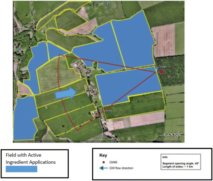
Well location, fields in well vicinity and product use history for a given year up-hydraulic gradient of the monitoring well (45–60 degree arc)

Groundwater characterisation
-
GLP sampling and analysis (limit of quantification 0.05 µg/L for all analytes, SANCO validated method) with collection of groundwater temperature, DO, redox, conductivity and water level.
Outputs
-
Results graphed temporally for each site and used alongside descriptive statistics to assess variability of residues amongst sites.
-
Boxplots indicate the centre, spread, skewness and outliers within the dataset to help evaluate groundwater quality spatially amongst national wells.
-
Elucidations conducted if national regulatory trigger exceeded.
-
Rolling averages indicate the long term quality of the groundwater temporally. Recommended for evaluating non-relevant metabolites.
-
Extrinsic vulnerability of sites compared to other EU locations for suitability in other Member States based on soil and weather.
Example III
Study type: Monitoring using nationally-owned wells within an Intensive agricultural area
Study objectives Determine the potential for a relevant metabolite common to multiple active substances to leach to shallow groundwater following intensive combined use of those substances. The substance in question is however also applied directly to soil in much larger quantities as a nitrification inhibitor with mineral or organic fertilisers.
Exposure assessment option: 4, for some sites 2, 3.
COMPOUND CHARACTERISTICS | |
Small, polar metabolite (biphasic DT50 ~ 1d/~ 60 d) | |
PROGRAMME OVERVIEW | |
Number of monitoring sites | 11 |
SITE CHARACTERISTICS | |
Target crop coverage | Cereals (grown in rotation with sugar beet) |
Product application criteria | Applications by farmers as required commercially, to fields in locations up-hydraulic gradient of well |
Retrospective/prospective | Retrospective |
SITE SELECTION CRITERIA | |
Wells chosen from existing monitoring networks belonging to public water supply wells | |
Significant historic findings of a non-relevant metabolite from a product used in sugar beet demonstrating connectivity to treated fields | |
Agricultural land use with target crops up-hydraulic gradient | |
Wells of good construction away from point sources and surface water features with relatively flat topography | |
Wells target shallow groundwater between 1–10 m below ground surface screened at top of saturated zone | |
Use of products up-hydraulic gradient | |
Fertiliser applications with the target substance as a nitrification inhibitor ruled out in farmer interviews | |
VULNERABILITY | |
Intrinsic vulnerability | Region selected for cereal cultivation in rotation with sugar beet. Typically sandy soils. Targeted to shallow, unconfined groundwater. Vulnerability demonstrated by findings of metabolite from product used in sugar beet |
CONNECTIVITY | |
Inferred from hydrogeological situation and well location | |
Expert knowledge by monitoring well owners | |
Detects of non-relevant metabolite and target substance in down-hydraulic gradient wells prove hydraulic connection to application area | |
SAMPLE FREQUENCY | |
Wells sampled every 3 months. Considered sufficient due to ubiquitous and frequent use of associated products | |
Well design selection criteria
-
Borehole log with strata described, water level, screen length.
-
Aquifer type and characteristics known.
-
Groundwater flow direction and velocity characterised and provided by well owners (Fig. 27).
Fig. 27 
Well location, fields in well vicinity and product use history (ca. 20 associated products surveyed) up-hydraulic gradient of the monitoring well

Groundwater characterisation
-
GLP sampling and analysis (limit of quantification 0.05 µg/L for all analytes) with collection of groundwater temperature, DO, redox, conductivity and water level.
Outputs
-
Time series concentration data showing temporal variability for the target substance.
-
Relevant product usage in the upstream area.
-
Range of different application patterns with similar hydrogeological situations.
Remarks
The study design was very much determined by the target molecule having multiple sources in agriculture (different active substances, fertiliser additive), which are subject to differing regulatory trigger concentrations in groundwater. This meant that extensive farmer interviews were intrinsic to the site selection.
A large proportion of potential monitoring sites were ruled out due to applications of the target metabolite molecule in its use as a nitrification inhibitor identified in the up-hydraulic gradient recharge areas.
Example IV
Study type: Prospective in-field monitoring using field leaching sites
Study objectives Prospective in-field monitoring of upper groundwater to determine leaching potential for a post-emergence herbicide used in a single crop. Sampling at intensively instrumented field sites with high leaching vulnerability.
Exposure assessment option: 2/3 (4)
COMPOUND CHARACTERISTICS | |
Relatively slowly degrading parent (DT50 77d) and two mobile metabolites. | |
PROGRAMME OVERVIEW | |
Number of monitoring sites | 3 |
SITE CHARACTERISTICS | |
Target crop coverage | Maize (pre- or early post-emergence) |
Product application criteria | Fields should not have received previous applications of product. Applications after well installation in spring/early summer according to normal application practices |
SITE SELECTION CRITERIA | |
Maize growing regions | |
Sandy soil with low organic carbon | |
Shallow groundwater (< 5 m below ground) | |
High precipitation | |
Flat topography without significant slope | |
Absence of surface water influences | |
INTRINSIC VULNERABILITY | |
Shallow groundwater, no confining layers, locations with relatively high rainfall, soils with higher sand content and low organic carbon | |
CONNECTIVITY | |
Tracer (KBr) applied with test substance to establish potential arrival of test substances at sampling points | |
SAMPLING | |
Wells sampled prior to application, 0.5 and 1 month after application, then monthly up to 48 months | |
Groundwater was sampled at a depth of 0.5 m below the current water table, using a peristaltic pump with low discharge to avoid excessive drawdown | |
Analysed for test substance, two metabolites and bromide tracer | |
SOIL CHARACTERISATION (optional) | |
Soil sampling and characterisation at multiple locations to 1 m depth. Texture, OC, pH for combined samples at each depth interval | |
Field design
-
12 in-field wells were installed (3 lines of 4 wells oriented at right angles to the main groundwater flow direction) at each ~ 1 ha. site with filter screens of 2 m length beginning above the groundwater table (to allow for increases in groundwater level above that found during installation).
-
Automated loggers for groundwater level were installed in four wells at each site.
-
Automated weather stations (precipitation, temperature) were installed at each site.
-
Application of the test substance according to GAP at the beginning of the study and cultivation of maize in the first season. Subsequently normal cultivation and agricultural activity.
Site characterisation and analysis
-
Soil sampling and characterisation at multiple locations to 1 m depth. Texture, OC, pH for combined samples at each depth interval.
-
Drilling profiles from well installation. Estimation of aquifer parameters (hydraulic conductivity, effective porosity) from aquifer material.
-
Recording of groundwater levels with data loggers.
-
On-site measurement of temperature and precipitation.
Outputs
-
Time-series concentration data at individual sites allow assessment of temporal variability.
-
Multiple wells per field allow assessment of local spatial variability.
-
Spatial averaging of localised measurements to assess leaching risk at the scale of a single field.
Remarks
This type of study design could also be considered for a field leaching study, but can be used for evaluating groundwater exposure under assessment options 2, 3 and 4. However in doing so, the local origin of the samples needs to be considered. Figure 28 shows results for the test substance from one sampling year. The results are quite typical for this type of study design; concentrations are low, or below LOQ at most times and locations beneath the field, with occasional isolated concentration peaks above the regulatory trigger (0.1 µg/L) in individual wells at some sampling events. Depending on the definition of the exposure assessment goal for which the study is being evaluated, such effects of localised heterogeneity may lead to differing regulatory conclusions.

Concentration time series for the test substance in individual wells at a field site during one study year
Example V
Study type: Prospective in-field monitoring using field leaching sites
Study objectives Determine the potential for the active substance and relevant metabolites to move to groundwater under commercial maize growing locations.
Exposure assessment option: 5, in some cases 4.
COMPOUND CHARACTERISTICS | |
Parent and relevant metabolites are highly mobile, relatively persistent in soil, (half-life of 20 d to 1 year depending on climate and soil type conditions) | |
PROGRAMME OVERVIEW | |
Number of monitoring sites | 6 |
SITE CHARACTERISTICS | |
Target crop coverage | Maize (pre- or early post-emergence) |
Product application criteria | Fields should not have received previous applications of product. Applications after well installation in spring/early summer according to normal application practices |
SITE SELECTION CRITERIA | |
Maize growing regions | |
Sandy soils | |
Water table between 1–4 m below ground surface | |
Field size more than 1 ha | |
Sites represented different intrinsic vulnerability characteristics e.g. OC content and climate by locating across several countries | |
INTRINSIC VULNERABILITY | |
Sites were selected with shallow groundwater, sandy soil with no confining layers and therefore considered conducive to leaching | |
CONNECTIVITY | |
Tracer (e.g., KBr) applied at the same time as the test item to understand the site and timeframe of movement through the soil profile | |
SAMPLE FREQUENCY | |
Wells sampled every month until desired information obtained or once tracer removed from well system | |
SOIL CHARACTERISATION | |
Terrestrial field dissipation (TFD) study conducted on the same site to determine the behaviour of the compounds in soil over time and to help contextualise the results observed from the field leaching study | |
Soil cores collected to determine soil properties in vadose and saturated zones. | |
Field design
-
Prior to product application, six clusters of monitoring wells were installed distributed around the four edges of the field. One cluster was installed within the field. Each cluster consisted of two wells (one shallow and one deep well) (Fig. 29).
Fig. 29 
Site design for one site in which three additional clusters were added along with deeper wells to the original clusters

Site characterisation and analysis
-
Water table measurements collected from each well prior to sample collection, allowing for the determination of groundwater flow direction over time.
-
During sample collection, measurement of groundwater physico-chemical characteristics (e.g. pH, electrical conductivity, dissolved oxygen content and water temperature).
-
Hydraulic conductivity (slug tests) of saturated zone measured to determine permeability.
-
On-site weather station installed and soil probe installed to determine soil moisture and temperature.
-
GLP sampling and analysis using SANCO validated method.
Outputs
-
Data plotted temporally for study duration at each site to understand the leaching behaviour of parent and metabolites.
-
Descriptive statistics used alongside temporal data to evaluate spatial differences between sites and wells within the same site.
-
Rolling averages indicate the long term quality of the groundwater over time both temporally and spatially across each site in study.
Example VI
Study type: Retrospective monitoring using existing wells and dedicated edge-of-field wells
Study objectives Determine the potential for the relevant metabolite to leach to shallow groundwater in areas with intensive target crop and regular usage of the active ingredient.
Exposure assessment option: 4, in some parts 5 and 6
COMPOUND CHARACTERISTICS | |
Mobile soil metabolite of a rapidly degrading parent. Mobility of metabolite is pH and OC dependent | |
PROGRAMME OVERVIEW | |
Number of monitoring sites | 124 |
Target EU countries | France, Italy, Poland, Czech Republic, Hungary, Romania |
Target groundwater FOCUS scenarios | Châteaudun Hamburg Jokioinen Kremsmünster Okehampton Piacenza Porto Seville Thiva |
SITE CHARACTERISTICS | |
Target crop coverage | Maize |
Product application criteria | Documented historic application of the target compound in the field directly upgradient to the sampling well |
Field size | Minimum of 1 ha |
SITE SELECTION CRITERIA | |
Target areas identified via vulnerability mapping of modelled mass flux (PEARL) | |
VULNERABILITY | |
Extrinsic vulnerability | Sites cover a wide range of percentile vulnerability modelled mass flux with proven applications of the target compound within at least 5 years |
Intrinsic vulnerability | Shallow groundwater (typically < 10 m below ground surface), vulnerable soil profile, typically no confining layers |
CONNECTIVITY | |
Connectivity was assumed by placing wells at the edge of treated fields with screens at the top of the saturated zone | |
SAMPLE FREQUENCY | |
Mainly quarterly, more frequently in France (2 month sampling intervals and additional sampling events at karst sites) | |
Field site design
Typically 20 monitoring sites were located in each of the countries. Where possible, existing wells from monitoring networks in Member States were included in the study (Fig. 30). The number was supplemented with dedicated edge-of-field monitoring wells that are screened in the upper section of the aquifer. At new well sites, two additional piezometers were installed to determine the local groundwater flow direction via triangulation. Groundwater depth was typically < 10 m. Soil characteristics were obtained at each site to aid in understanding movement through the soil profile.

Spatial distribution of monitoring wells with the country specific vulnerability assessment of modelled mass flux
The monitoring design was somewhat different in France, with 24 monitoring sites in representative areas. Deeper wells, raw water from drinking water wells and karst spring locations were included to cover a wider range of settings. Groundwater flow direction at each site was determined from contour maps or hydrogeological catchment delineation. Samples were collected every 2 months from each site, with additional sampling events at karst sites.
Groundwater sampling and analysis
-
Samples shipped chilled to avoid degradation.
-
GLP sampling and analysis using SANCO validated analytical methods.
-
Limit of quantification of 0.05 µg/L.
Site characterisation and analysis
-
During sample collection, measurement of groundwater physico-chemical characteristics (e.g., pH, electrical conductivity, dissolved oxygen content and water temperature).
-
Hydrochemical parameters determined for one groundwater sample for each site.
-
Slug tests to determine the hydraulic conductivity of the local saturated zone.
-
Drilling profiles from well installation.
Outputs
-
Residue concentration data of 1100 samples from 124 monitoring sites (study is still ongoing).
-
Tabulation of detailed product use data for the field upgradient to the monitoring well, for each site.
-
Assessment of the sources of residues for wells in which the regulatory trigger value was exceeded (some sample contamination identified).
Example VII
Study type: In-field retrospective monitoring
Study objectives Determine the presence of the active substance and its metabolites in shallow groundwater under intensive commercial maize fields after regular active ingredient uses.
Exposure assessment option: 2
COMPOUND CHARACTERISTICS | |
Rapidly degrading (microbial) parent (DT50 < 2d), mobile relevant metabolite (DT50 of 20d), mobile non-relevant metabolite (DT50 of 20d) | |
PROGRAMME OVERVIEW | |
Number of monitoring sites | 10 |
SITE CHARACTERISTICS | |
Target crop coverage | Maize |
Product application criteria | Normal commercial application |
Retrospective/prospective | Retrospective |
SITE SELECTION CRITERIA | |
A vulnerable field at least 10 ha in area which had been treated in at least three of the past 5 years with the active ingredient under study | |
Weather station with precipitation data available nearby | |
Groundwater less than 8 m beneath the field surface | |
Acceptability of candidate fields agreed to by regulators. Field characteristics verified during well installation | |
Potential sites located using GIS information and product sales records and then calls were made to growers to determine acceptability of the sites and willingness to cooperate. Calls indicating promising sites were followed up with site visits | |
A single well was installed in the middle of the field with the well screen located at the top of the saturated zone. Wells were installed during the winter to prevent interference with crop growing activities and removed prior to planting the next season | |
VULNERABILITY | |
Intrinsic vulnerability | Sites selected by the site selection process represented high intrinsic vulnerability within the label constraints in the use area under study. Vulnerable surface and subsoils within conditions allowed by the product label were chosen |
CONNECTIVITY | |
Connectivity was assumed by placing wells in the middle of treated fields with screens at the top of the saturated zone | |
SAMPLE FREQUENCY | |
Wells were sampled one time (potential for a single follow-up sample to confirm any detections) and wells were then removed to prevent interference with crop growing activities | |
Site and groundwater characterisation
-
Boring logs obtained for each well.
-
GLP sampling and analysis with measurement of the groundwater depth below ground surface and measurement of groundwater temperature, pH, and conductivity.
Outputs
-
Concentrations of parent and metabolites in shallow groundwater in the sample collected at each of the ten sites with at least three applications in the last 5 years.
Example VIII
Study type: Prospective in-field monitoring using a field leaching site
Study objectives
-
Determine the potential for the active substance and relevant metabolites to move vertically and horizontally to groundwater under commercial potato growing conditions in the Netherlands.
-
Determine the degradation characteristics of the active substance and its metabolites in the unsaturated and saturated zones.
Exposure assessment option: 5
COMPOUND CHARACTERISTICS | |
Parent and relevant metabolites are highly mobile, relatively persistent in soil, (half-life of 0.5–2 months depending on climate), degradation in groundwater dependent on temperature, pH, and redox potential (compound degrades relatively rapidly under anaerobic conditions) | |
PROGRAMME OVERVIEW | |
Number of monitoring sites | 2 |
SITE CHARACTERISTICS | |
Target crop coverage | Potatoes/tubers in two potato growing regions in the Netherlands |
Product application criteria | Fields should not have received previous applications of product. Applications after well installation in spring according to normal application processes which includes soil incorporation, resulting in residues down to a depth of 0.22 m |
SITE SELECTION CRITERIA | |
Sandy soils | |
Water table between 1–2 m below ground surface | |
Fields agreed with appropriate regulatory agency | |
INTRINSIC VULNERABILITY | |
Sites had sandy soils with a shallow water table. | |
CONNECTIVITY | |
Residue plume tracked through field. No tracer applied because residues used instead. | |
SAMPLE FREQUENCY | |
Sample wells at approximately monthly intervals for 15 months, then at increasing intervals guided by results from previous sampling intervals | |
Continue sampling until desired information is obtained (one site was continued for 7 years and the other for 10 years) | |
SOIL CHARACTERISATION (required to achieve study objective: to determine degradation rate in the unsaturated zone, otherwise soil characterisation optional) | Soil samples collected prior to treatment, immediately after application, and at 1, 2, 4, 6, 8, 10, 12, and 14 months after application Soil cores consisted of a single sample of 0–0.3 m for sampling immediately after application and divided into strata of 0–0.3, 0.3–0.6, 0.6–1.2 m, and 1.2–1.8 m. The deepest strata may not be possible at sites with shallow water tables |
Field design
-
Prior to product application, six clusters of monitoring wells with 0.3 m screens installed at each site (Fig. 31). Each cluster consists of two or three wells, with one well located just below the water table and the next at about 1.5 m intervals allowing vertical plume tracking.
Fig. 31 
Design for one site with three additional clusters added along with deeper wells to the original clusters (subplots identified by Roman numerals, well clusters by Arabic numerals)
-
Horizontal groundwater movement regarded as quite slow in these areas in the Netherlands, thus initially two well clusters located in the middle of the future-treated area, with wells located at the edge-of-the treated area.
-
Wells installed as necessary to follow the residue plume both vertically and horizontally. At one of the locations, wells were installed up to 5.8 m deep and at the other location up to 25 m below ground surface.

Groundwater characterisation
-
Water table measurements collected from each well prior to sample collection, allowing for the determination of groundwater flow direction as a function of time.
-
During sample collection, measurement of pH and conductivity.
-
In this particular case, occasional measurements of redox potential were recorded because of its effect on degradation rate in groundwater.
Outputs
-
Degradation rate of parent and metabolites as a function of depth in soil at two different study sites.
-
Time series data at two different study sites to show vertical and horizontal movement of parent and metabolites in groundwater.
-
Outputs from multiple wells at two different study sites to show the temporal and spatial variability of residues.
-
Redox potential and its association with degradation rate in groundwater evaluated through statistical tests.
Example IX
Study type: Analysis of publicly available monitoring data
Groundwater monitoring data for compound A were obtained from the ADES data base (http://www.ades.eaufrance.fr). Compound A has been registered and used in France since 1977–1978. The data were downloaded from the ADES database on 18 March 2014 and includes analysis from 7 April 2004 to 18 December 2013. The total number of analysis available for compound A was 55,861, measured in 12,173 different wells. The distribution of the wells where compound A was analysed in France is shown in Fig. 32.

Well location of wells (blue dot) with available monitoring data for compound A
As compound A is almost exclusively used on oil seed rape (OSR), only the wells located in areas where OSR is cropped were selected for further analysis. This was done to remove false negatives (in areas where OSW is not cropped, compound A was most probably analysed in a multi-residue method and was not detected simply because it was not used in the area of the wells).
The distribution of the wells where compound A was analysed in the OSR cropping area is illustrated in Fig. 33. The OSR cropping area is defined as the area representing 86.4% of the cumulative OSR acreage using the 2010 agricultural statistical data from the French Ministry of Agriculture at canton level and include cantons where OSR is greater than 5% of the arable land (http://www.agreste.agriculture.fr). The total number of analysis available for compound A in the OSR cropping area was 22,853, measured in 4171 different wells (Table 4).

Location of groundwater wells where compound A was analysed (blue and green dots) in the oilseed rape cropping area
From the 22,853 analyses of compound A in the OSR cropping area, 367 analyses showed detects above the limit of quantification (LOQ) in 189 different wells (i.e. 1.6% of the analyses located in 4.5% of the wells in the OSR cropping area). The LOQ reported in the ADES database for each individual analysis were ≥ 0.001 µg/L. Only the results classified as validated in the ADES database were used in the evaluation.
A total of 110 analyses of compound A over 46 different wells were above the environmental quality standard of 0.1 µg/L as set up in the groundwater directive (EU Commission 2006). These wells are represented by the green dots in Fig. 32. They represent 0.5% of the total analysis conducted in the period 7 April 2004 to 18 December 2013 in the OSR cropping area, and correspond to 1.1% of the wells located in the OSR.
For the 46 different wells with at least one sample with a concentration of compound A above 0.1 µg/L, the time series of analytical residue data were plotted to differentiate wells with a single analysis from wells with multiple analyses and to differentiate wells with a single sporadic detect from sites with regular detects. As an example, the time series of concentrations from five wells are presented in Fig. 34.

Examples of time series concentrations for compound A in five wells (concentrations are reported in µg/L)
In discussions with national authorities, 16 wells of the 46 wells with concentrations in at least one sample above 0.1 µg/L were selected for further field investigation and additional monitoring. The aim of the additional field investigation and monitoring was to identify the reason for the concentrations of compound A in those wells (either due to well catchment area or point source contamination) and to identify any potential need for specific mitigation measures to reduce the frequency and/or magnitude of the observed concentrations.
Appendix 3: Catchment surveys
When conducting monitoring studies, information on product usage and farming practices need to be obtained during site selection and at various times during the study. For in-field and edge-of-field studies with monitoring wells located at the top of the water table, this may involve only a single field (and perhaps an upgradient field), but in other circumstances information on a number of fields may be needed. This will normally involve a conversation with the grower during the site selection/study initiation phase and yearly updates afterwards. In addition, when existing wells are used, a careful examination of the well should be conducted before it is included in a sampling programme.
Initial survey
The nature of the survey will depend of the specific objectives of the study. If the study is retrospective, then information on the previous use of the product under study will be essential for site selection. For a prospective study, past use data is needed but is not as critical for site selection
The main areas where information may be needed include:
-
Location and size of field.
-
Crops grown during each of the past 3–5 years.
-
The use of the product under study during the past 3–5 years.
-
Method of application.
-
Dose rates (if available).
-
Timing (exact dates if available, otherwise a rough estimate will usually be sufficient.
-
-
Presence of tile drainage.
-
Irrigation practices.
-
Type of irrigation.
-
Number and amount (if available).
-
-
Depth to groundwater (if available).
-
Soil type (often from data bases rather than the grower).
-
Weather conditions (often from data bases rather than the grower).
-
Soil cultivation practices (if relevant).
-
Fertilisation practices (if relevant).
Follow-up surveys
When prospective studies are being conducted, annual follow-up surveys after the initial visit may be needed to provide information on the crop and applications during the previous year.
Well inspections
A site survey may also include an examination of an existing monitoring well. This topic is included in Sect. 5.
Appendix 4: List of available methods for vulnerability mapping
Name of the model/method | Description | Area modelled | Comment | References |
|---|---|---|---|---|
Process-based methods | ||||
EuroPEARL | Spatially distributed model of PEARL | Europe | Tiktak et al. (2004) | |
EuroPEARL2012 | Spatially distributed model of PEARL | Europe | Waterborne and Syngenta: Poster B21, York conference 2013 | |
GeoPEARL | Spatially distributed model of PEARL | Netherlands, Austria | ||
SuSAP—PELMO (version 3.0) | Spatially distributed model of PELMO | Lombardy Veneto | Life Environment Project (LIFE98/ENV/IT/00010) | |
MACRO | England and Wales | Holman et al. (2004) | ||
MACRO SE | ||||
GEORGE | Pesticide leaching model based on PCRaster framework | |||
Statistical methods | ||||
MetaPEARL | Metamodel of EuroPEARL. Multiple linear regression model that mimics the behavior of EuroPEARL | Europe | Easy applicable to GIS data | Tiktak et al. (2006) |
Fuzzy logic approach | Dixon (2005) | |||
Bayesian methods | Based on the weight of evidence approach (using location of known contamination as training set) | Masetti et al. (2007) | ||
Index methods | ||||
DRASTIC | The DRASTIC parameters (depth to water, net recharge, aquifer media, soils, topography, impact of vadose zone, and hydraulic conductivity) form the vulnerability rating or DRASTIC index | USA, Turkey, Japan, Romania | Aller et al. (1987), EPA | |
EPIK Epikarst, Protective cover, Infiltration, karstic network) | Like DRASTIC it can be classified as PCSM method (see note on index methods). Mainly focused on karst systems. Based on additive parameters which are weighted by different coefficients | Spain (Andreo et al. 2006); South German (Neumann 2008) | Neukum et al. (2008) | |
SINTACS | It is an adaptation of DRASTIC to Italian conditions (infiltration factor instead of net recharge factor) | Italy | Civita and De Maio (2004) | |
Irish approach | The approach can be classified as MS (see note on index methods) and produces maps at the scale of 1:50,000 with four classes of vulnerability | Ireland | ||
SNIFFER | MS method based on soil and subsoil properties, lithology and depth to groundwater | Ball et al. (2004) | ||
GLA (Geologisches Landsamt) | RS method (see note on index methods) based on the protective capability of the three layers (topsoil, subsoil and rock) overlying groundwater | Spain | Lamelas et al. (2007) | |
COP | RS method which considers several parameters (Concentration of flow, Layers, Precipitation, Karst network) | Spain | Vias et al. (2006) | |
SINTACS + IPNOA | Based on DRASTIC methodology (see above) to produce a vulnerability map and integrated with a control factor based on soil organic matter to produce a hazard (pericolosità) map | Toscana Emilia Romagna | (1) Civita and De Maio (2000) (2) Padovani and Trevisan (2002) | |
SINTACS + PEARL | Two level mapping: (1) contamination risk map which combines an Intrinsic vulnerability map based on SINTACS (DRASTIC) and an Intensive agriculture zones map; (2) active substance specific/potential vulnerability map based on PEARL | Calabria | ||
TOT (time of travel) + soil capacity to protect aquifers | Combining two maps (1) time of travel of a water transported contaminant; (2) soil capacity to protect aquifers (soil attenuation capacity) | Piemonte | (1) Hollis (1991) (2) Bove et al. (2003) | |
Appendix 5: GIS data available at european level for vulnerability mapping
The situation regarding pan-European GIS data for use in creating vulnerability maps is clear with a wide range of comprehensive electronic datasets available for soils, climate, cropping, land use, water quality etc. available from the EU Joint Research center, ISPRA, Italy (MARS climate data, European Soils Bureau) and the European Environment Agency, Copenhagen, Denmark (Corine land use, WISE and WATERBASE water quality data). These data can be used to prepare vulnerability maps at pan-European and probably at national scale with a reasonable degree of confidence.
There are a number of Geoportals available which are always a good starting point to search, view and access different types of GIS datasets. Lists of these web portals including some useful datasets are put together in the following table. However, we make no claim that the list is complete.
Type of information | Name | Source | Data type | Publication date | Weblink | Description |
|---|---|---|---|---|---|---|
Geo-web portals | ||||||
Geo-portal | INSPIRE Geoportal | Search, view, and access to GIS data of European authorities | ||||
Soil data on European level | ||||||
Different geo-spatial data | GeoNetwork—database for GIS datasets, satellite imagery and related applications | |||||
Statistical data | EUROSTAT | http://epp.eurostat.ec.europa.eu/portal/page/portal/eurostat/home | ||||
Statistical data | GISCO | Vector | 2010 | http://epp.eurostat.ec.europa.eu/portal/page/portal/gisco_Geographical_information_maps/introduction | Shapefiles of NUTS areas | |
Geology | OneGeology | Search, view, and access to geological spatial data | ||||
GIS data sets | ||||||
Soil, climate, landuse | EFSA spatial data | JRC | Raster, 1 km | 2013 (ver. 1.1) | Comprehensive and homogeneous set of raster data provided for spatial analysis and modelling in context of PPP registration in EU-28. Data sources: ESDB, HWSD, Worldclim, CAPRI, Corine) | |
Soil | European Soil Data Base ESDB | JRC | Vector or Raster | 2006 (ver. 2.0) | ESDB contains 1:1M soil map of Eurasia with soil map units and corresponding soil properties database (partly based on pedotransfer rules) | |
Soil | LUCAS topsoil survey | JRC | Vector (point) | 2013 | Laboratory analysis of physical and chemical properties of 19,967 geo-referenced samples. Cover: EU28 without RO/BG/HR | |
Soil | Soil pH in Europe | JRC | Raster, 5 km | 2009 | Estimated soil pH values across Europe from a compilation of 12,333 soil pH measurements from 11 different sources, and using a geo-statistical framework based on Regression-Kriging | |
Soil | SPADE-2 | JRC | Vector (point) | 2006 | Soil profile characterisation for ESDB soil typological units (STUs) | |
Soil | OCTOP | JRC | Raster, 1 km | 2003 | http://eusoils.jrc.ec.europa.eu/ESDB_Archive/octop/octop_data.html | Topsoil organic carbon content in the surface horizon of soils in Europe |
Soil | OCTOP | JRC | Raster, 1 km | 2003 | http://eusoils.jrc.ec.europa.eu/ESDB_Archive/octop/octop_data.html | Topsoil organic carbon content in the surface horizon of soils in Europe |
Soil | Harmonized World Soil Database HWSD | FAO, IIASA, ISRIC, ISSCAS, JRC | Raster, 30 arc-second | 2012 | http://webarchive.iiasa.ac.at/Research/LUC/External-World-soil-database/HTML/ | Global soil map with variety of soil attribute data attached to the map |
Land cover | CORINE Land Cover | European Environmental Agency | 2006 | http://www.eea.europa.eu/data-and-maps/data/clc-2006-vector-data-version-2 | Inventory of land cover in the EU Scale of 1:100 000 | |
Climate + Meteo | MARS | JRC | JRC MARS unit provide different meteorological time series data (AGRI4CAST interpolated meteo data 25 km; FOODSEC 10-days periods data) | |||
Hydrogeology | Depth to groundwater table | GLOWASIS | 2013 | https://glowasis.deltares.nl/thredds/catalog/opendap/opendap/Equilibrium_Water_Table/catalog.html | Global map of groundwater table depth (Fan et al. 2013) | |
Appendix 6: Time of flight modelling methodology
This appendix presents one possible approach to time of flight modelling for estimating the time from application of a substance to arrival of a solute peak at a specified evaluation depth using a leaching model. In this case, an example substance is used in an adaptation of a standard FOCUS scenario to demonstrate the principal of the methodology. If such an approach is used to estimate leaching times or address related questions for a specific monitoring location, it is necessary to parameterise the scenario with a site-specific soil profile and the appropriate meteorological and cropping data.
Introduction
Time of flight (ToF) analysis is a means to estimate the time taken for active ingredients and their metabolites to reach specific depths in soil after application to the soil surface. This estimate of ToF can be used to define how far back the application history for a particular site needs to be known. It can also demonstrate that a product would be expected to have reached a well at a specific depth by a certain time. Prediction of the width of a solute peak can also be used to determine a sampling schedule designed to capture peak residues.
ToF modelling methodology
FOCUS scenario
The FOCUS modelling guidelines provide a standardised framework for estimating residues at 1 m soil depth. Several scenarios are available covering a range of weather and soils appropriate to agronomic conditions in the EU28.
The FOCUS Hamburg scenario was chosen as the basis for the ToF modelling because the scenario frequently yields the highest groundwater predicted environmental concentrations (PECs) and therefore represents the type of worst-case leaching sites selected in monitoring studies.
Soil profile
The standard FOCUS Hamburg scenario soil profile extends to a depth of 4.5 m. However, groundwater monitoring wells are frequently installed in areas where the groundwater depth is > 4.5 m. The Hamburg soil profile was therefore extended to allow ToF estimates for depths > 4.5 m (Table 5; Fig. 35). This was achieved by increasing the depth of the 6th horizon from 3.5 to 4 m, and adding a 7th horizon, 7 m deep, below this, thus bringing the total depth of the modified soil profile to 12 m. The newly added seventh soil horizon has exactly the same soil characteristics as the sixth horizon. In the standard Hamburg scenario the sixth horizon is 100% sand with zero organic carbon content; therefore no arbitrary decisions were required regarding the variation of soil organic matter at depths beyond those provided by FOCUS.

Conceptual model of the extended soil profile, with target depths of 1 m, 5 m, and 10 m highlighted
In line with the standard FOCUS Hamburg scenario, the groundwater level was set at 1 m below the target depth being investigated. For example, for a target depth of 1 m the groundwater level was set at 2 m, whereas for a target depth of 5 m the groundwater level was set at 6 m (Fig. 35).
Increasing the dispersion length used in the extended soil profile horizons was necessary since the parameter is scale dependent. The dispersion length within a FOCUS scenario is set at 0.05 m which is appropriate for a 1 m target depth, and this is kept consistent across the first five soil horizons. The dispersion length in the sixth horizon, which covers a depth of 1–5 m, was set at 0.25 m, and the dispersion length in the seventh horizon, covering a depth of 6–12 m, was set at 0.5 m. Standard assumptions with respect to the variation of degradation rate with depth assumed by FOCUS were used.
Target depth
A target depth of 1 m provides a convenient reference with standard FOCUS modelling, however it is unlikely that a monitoring study would install a well screen at this depth. It is also likely that the length of the well screen would be at least 1 m making 1 m evaluation depth inappropriate. ToF analysis therefore focused on a target depth of 5 m. The 5 m target depth was assumed to be the most relevant in support of a monitoring study in shallow groundwater, as this depth of evaluation would likely be more typical of the position of a well screen in such a study.
Meteorological variation
Standard regulatory modelling, utilising FOCUS scenario assumptions, simulates compound application events in sequential years. This can yield concentration time-series which are difficult to interpret with respect to quantification of travel time from a specific application. Therefore, the modelling approach adopted in the ToF analysis was to model single applications. A ToF simulation consists of a single application event in a 26 years period, consisting of a 6 year warm-up period, an application year and 19 subsequent years without application. This produces a distribution of 20 different ToF time-series representing the variation in Hamburg soil under Hamburg weather conditions (Fig. 36). The temporal specification of each of the 20 simulations is summarised in Table 6.

An example of the distribution of time of flight (ToF) time-series generated for a specific metabolite
Time of flight definition
Time of flight and earliest arrival time
The ToF has been defined as the time taken from application at the soil surface for the peak PECmax to arrive at the target depth. However, in a situation where the solute concentration profile shows multiple peaks, which is often the case at shallower target depths, this can result in inconsistent estimations of the peak arrival time that suggest a faster ToF to 5 m than to 1 m (Fig. 37). An alternative approach is to define the earliest arrival time (EAT) as that when 10% of the area under the solute curve has been reached at the target depth (Fig. 38).

An example of an active ingredient which has a multi-peak concentration time-series. The use of the PECmax as an estimate of pesticide arrival at the target depth would be inaccurate

Example concentration time-series for a single application, illustrating how the earliest arrival time (10% of the area under the curve—AUC), expected peak window (10–60% AUC), and the months at target concentration (MTC) are defined
Expected peak window
By its nature, the point at which 10% of the area under the solute curve is reach is an instantaneous event. It was therefore necessary to define an expected peak window (EPW), which would be broadly representative of the period of time during which the maximum solute concentrations would be expected to be observed. This period was defined as the time take from EAT (10% area under the curve) to when 60% of the area under the solute curve to be reached (equating to 50% of the area under the curve; Fig. 38).
Months at target concentration
The months at target concentration (MTC) is a measure to use to ensure that concentrations within a certain percentage of the PECmax will be observed with a set sampling window. It is taken as the number of months within the defined target concentration window when concentrations are at or above the 70% of the PECmax (Fig. 38).
Reporting
An R language ToF Analysis Code was developed and is provided in the supplemental information. This code produces all summary statistics and figures required for ToF reporting:
-
LoQ is specified as a input parameter.
-
Percentages used in the area under the curve method are specified as a input parameters.
-
Code includes additional outputs:
-
A flag if the PECmax is outside the target concentration window.
-
If it is the code will tell you if the peak occurs before or after Expected Peak window and by how many months.
-
The number of months the concentration is above the target concentration (set as a percentage of the peak) within the target concentration window is also reported.
-
Reporting requirements are as follows:
-
Earliest arrival time for each of the individual simulation years are reported in table format along with the minimum, maximum and median arrival time.
-
Tables are written to excel file with the name specified by the code input parameter “SumRE”.
-
-
Regulatory decisions are based around the median earliest arrival time. This was adopted as opposed to mean to reduce bias by outliers.
-
The code also reports to the time to initial detect (> 0) and the time to detects at the LoQ, which are optional in final reporting.
-
The expected peak window for each of the individual simulation years are reported in table format along with the minimum, maximum and median.
-
The months at target concentration (MTC) within this window can also be reported.
-
If being used to inform sampling strategy, regulatory decisions should be based around the minimum MTC. It is assumed that this is the worst case and a sampling schedule based on this would be highly likely to detect concentrations close to the maximum concentrations.
-
-
The code can also produce cumulative frequency plots of the earliest arrival time results.
-
The name given to all plots is specified by the “CFPlotAll” parameter in the code.
-
-
Time-series plots of the concentration and mass flux data can also be produced.
-
Set code input parameter to “1”.
-
Appendix 7: Examples of coupling leaching models with hydrogeological models
This appendix presents two posters (Miles 2014; Sur et al. 2011) showing examples of leaching models coupled with hydrogeological models.


Appendix 8: Glossary of terms
Aquifer
Geological water-bearing formation (bed or stratum) of permeable rock, or unconsolidated material (e.g., sand and gravels) capable of yielding significant quantities of water.
Aquifer scale monitoring
Monitoring of all wells from the same groundwater body. The number of wells included in such monitoring may have been developed to address the Water Framework Directive or other national objectives. A link needs to be established between treated crops and the groundwater body.
Bailer
Sampling device (typically stainless steel tube) used to lower into a well or borehole to remove water.
Bank filtration
Infiltration of surface water, usually from a river system, into a groundwater system induced by water abstraction close to the surface water (e.g. a river bank).
Borehole
See well borehole.
Casing
Tubular retaining structure, which is installed in a drilled borehole or excavated well, to maintain the borehole opening.
Catchment
Area of land where all surface water from rain, melting snow, or ice converges to a single point at a lower elevation, usually the exit of the basin, where the waters join another body of water, such as a river, lake, reservoir, estuary, wetland, sea, or ocean.
Down gradient
Direction that groundwater flows; similar to “downstream” for surface water.
Edge-of-field scale monitoring
Groundwater monitoring where sampled well(s) are adjacent to but not always surrounded by treated crops. A link between the treated crops and groundwater (especially when shallow) can be made by considering the groundwater flow. The wells may already exist, or may use dedicated wells installed on site.
False negative
Substance of interest is not detected, but the sample is not related to the use of the substance (e.g. taken from where the substance has never been used, or sampled before the substance had time to reach groundwater). Could also arise because the LOD/LOQ is not adequate for the purpose, or due to poor sample handling (e.g. degradation during transport/storage).
False positive
Substance of interest is detected, but the result cannot (or should not) be used in the evaluation because the result cannot be related to the agricultural use of the substance (e.g., contamination during sampling or analysis, faulty analytical method). A finding of residues resulting from a former application or other sites if may also be considered a false positive it is wrongly attributed to the current site or application.
Field leaching
Research type (usually prospective) study conducted at field scale with carefully controlled agricultural operations, e.g. application, under supervision of the researcher.
Fractured rock
Any separation in a geologic formation, such as a joint or a fault that divides the rock into two or more pieces. A fracture will sometimes form a deep fissure or crevice in the rock, commonly caused by stress exceeding the rock strength, causing the rock to lose cohesion along its weakest plane. Fractures can provide high permeability for water movement. Highly fractured rocks make good aquifers since they may possess both significant permeability and fracture porosity.
Groundwater
The definition of groundwater provided in Article 2 of Directive 200/60/EC is “all water which is below the surface of the ground in the saturation zone and in direct contact with the ground or subsoil.
Groundwater monitoring
General term used to cover any type of monitoring, e.g. public, in-field, edge-of-field, catchment and aquifer scale monitoring.
In-field scale monitoring
Groundwater monitoring where sampled well(s) are in very close proximity to and are surrounded by treated crops. A link between the treated crops and groundwater (especially when shallow) can implicitly be assumed. The wells may already exist, or may use dedicated wells installed on site.
Infiltration
Process by which water enters and moves through the soil horizon. It can occur via gravity or capillary action.
Intrinsic vulnerability
Vulnerability which takes into account the characteristics of an area (hydrogeology, soil, climate, etc.), but is independent of the nature of the contaminants.
Karst (karstic)
Landscape topography formed from the dissolution of soluble rocks such as limestone, dolomite, and gypsum, and characterised by underground drainage systems with sinkholes and caves.
Lance
A filter screen placed on a pipe that is driven into the saturated zone or placed in pre-drilled hole. The lance is attached to a vacuum bottle or suction pump for collection of a sample. This is also often referred to as a sampling lance or suction lance.
Metabolite
A biotic or abiotic degradation product formed from the active substance or a degradation product of the active substance (see also definition for relevant/non-relevant metabolite).
Packer
Device or material that inflates or expands for temporarily isolating specified vertical sections within boreholes to allow groundwater sampling from discrete zones or locations within the borehole or aquifer.
Pedoclimatic
Pertaining to soil and climate.
Perched water table
Groundwater supported by a zone of material of low permeability located above an underlying main body of groundwater. If a perched water table’s flow intersects the surface, at a valley wall for example, the water is discharged as a spring.
Permanent water table
Water table present continuously throughout the year.
Permeability
Ability to transmit water. Such water may move through the matrix or through joints, faults, cleavage or other partings. Permeable materials, such as gravel and sand, allow water to move quickly through them, whereas impermeable materials, such as clay, don’t allow water to flow freely.
Piezometer
Device consisting of a tube or pipe with a porous element or perforated section (surrounded by a filter) on the lower part (piezometer tip), which is installed and sealed into the ground at an appropriate level within the saturated zone for the purposes of water level measurement, hydraulic pressure measurement and/or groundwater sampling.
Point source
Source of contamination not resulting from proper agricultural use, e.g. spillage or equipment washings.
Preferential flow
Uneven and often rapid movement of water through soil via cracks, worm holes or root holes, allowing much faster transport of contaminants to the underlying groundwater. Not typically a leaching process.
Prospective monitoring
Monitoring focusing on an active substance or its metabolites resulting from applications made after the installation of the wells or after the initiation of the monitoring programme (if existing wells are used).
Public (general) monitoring
Routine monitoring carried out by national bodies and water authorities etc. often through multi-residue methods.
Recharge (groundwater)
Inflow of water to a groundwater body from the surface, e.g., precipitation, and its movement to the water table is one form of natural recharge.
Relevant/non-relevant metabolite
According to Sanco/221/2000-rev. 10 (25 February 2003) and refers to a metabolite which has the potential to leach to groundwater, and which has comparable biological activity to the active substance, or has certain toxicological properties. Conversely true for a non-relevant metabolite.
Retrospective monitoring
Monitoring focusing on an active substance or its metabolites resulting from historical applications made prior to the installation of monitoring wells or before the initiation of the monitoring programme (if existing wells are used).
Residue plume
Volume of contaminated groundwater that extends downward and outward from a specific source; the shape and movement of the mass of the contaminated water is affected by the local geology, materials present in the plume, and the flow characteristics of the groundwater.
Saturated zone
An area beneath the soil surface in which the pore spaces of the formation are completely filled with water.
Screen (well)
Keeps sand and gravel from the gravel pack out of the well while providing ample water flow to enter the casing. Water enters the well through perforations or openings in the screen. Wells can be screened continuously along the bore or at specific depth intervals.
Specific vulnerability
Vulnerability regarding a specific nature of the contaminants, e.g. environmental fate properties, use pattern.
Tile drain
Network of subsurface pipes installed to allow subsurface water to move out from between soil particles (especially clay) and into the tile line. Water flowing through tile lines is often ultimately deposited into surface water (ditch, pond, stream) at a lower elevation than the source.
True negative
Substance of interest is not detected and the sample is related to the use of the substance.
True positive
Substance of interest is detected and the result can be used.
Unsaturated zone
An area beneath the soil surface in which the pore spaces of the formation are not totally filled with water
Water table
Top of the water surface in the saturated part of an aquifer. Depth at which soil pore spaces or fractures and voids in rock become completely saturated with water.
Vadose zone
See unsaturated zone.
Vulnerability
Sensitivity of a groundwater system to contamination.
Well borehole
A hole sunk into the ground, either by drilling (boring) or digging, to obtain groundwater or for observation of the water table or measurement of water properties.
Well (groundwater)
Hole, shaft or excavation created in the ground by digging, driving, boring, or drilling down to access groundwater in underground aquifers. Most wells are vertical but they may also be horizontal or at an inclined angle.
Rights and permissions
Open Access This article is distributed under the terms of the Creative Commons Attribution 4.0 International License (http://creativecommons.org/licenses/by/4.0/), which permits unrestricted use, distribution, and reproduction in any medium, provided you give appropriate credit to the original author(s) and the source, provide a link to the Creative Commons license, and indicate if changes were made.
About this article

Cite this article
Gimsing, A.L., Agert, J., Baran, N. et al. Conducting groundwater monitoring studies in Europe for pesticide active substances and their metabolites in the context of Regulation (EC) 1107/2009. J Consum Prot Food Saf 14 (Suppl 1), 1–93 (2019). https://doi.org/10.1007/s00003-019-01211-x
Published:
Issue Date:
DOI: https://doi.org/10.1007/s00003-019-01211-x